CONSTRUCTING DEVELOPMENT SHAPES WITH MATHEMATICS

The construction of 3-D models from pieces from flat cardboard or thin sheet metal requires some mathematical and geometrical application. Starting with simple 3-D forms, we can calculate the shape of the flat 2-D object needed to make it. The flat shape is known as a DEVELOPMENT.

Supplies

Squared or graph paper

Ruler & pencil

Protractor

Drawing Compasses

French curves or Engineering spline ( optional )

Scissors & glue

Scientific electronic calculator or spreadsheet software ( Excel, Open Office, etc )

Thin cardboard, 360 gsm or similar ( empty breakfast cereal boxes are ideal )

Thin sheet metal ( eg, from aluminium drink cans, or heavy aluminium foil baking trays )

Step 1: PRISM

Take the case of a triangular right angled prism as shown in the diagram. Its development is simply a combination of its 5 faces, connected to produce the prism when folded along the edges.
For prisms which are not equilateral triangles at their base, each side of the base will require a rectangle which is of height H and length equal to the length of the base side. This is illustrated for the right trapezoidal prism shown. Generally speaking, developments for objects with plane sides are relatively simple to construct by measuring the dimensions of each face and combining them into a single 2-D shape. The faces need not be rectangular; triangles, parallelograms and trapeziums can all be used in the construction of the development. Objects with curved surfaces present more of a challenge, and some of these will be examined below.

Step 2: CYLINDER

Given the height of cylinder = H and diameter = D, the required shape will be a rectangle with sides H x πD, with πD being the circumference of the circular section. In order to produce a cylinder in cardboard, the development needs to be rolled around some other cylindrical object of similar diameter before glueing the joining tab.

Step 3: CONE

Imagine a cone being rolled around on a flat surface. The apex will remain in a fixed location, while the base will trace out a circular arc on the surface, with a length equal to the circumference of the cone's base. This generates the development for the cone, which is a sector of a circle with radius R and sector angle θ.

To calculate the dimensions of the development, first the slant height of the cone must be found from Pythagoras' theorem, ie R = √ [ H^2 + ( D/2 )^2]. The sector angle θ is found from the formula θ = D x ( 180 / R ), which gives θ in degrees. Draw the arc with compasses set to a radius of R .

Step 4: TRUNCATED CONE

A cone which is cut off by a plane parallel to its base is said to be truncated ( also called a FRUSTUM, Latin for a fragment ). Its development will be part of a circular sector bounded by two arcs with a common centre. The length of each arc will be equal to the circumference of the cone at its base and at the height of the intersecting plane. Firstly the apex angle of the cone needs to be found from the right triangle in the diagram, ie α = tan-1 [ ½ ( C – D ) / H ]. The full slant height of the non-truncated cone can then be found from R2 = ½ C / sin α. The hypotenuse of the right triangle in the diagram is H / cos α, which allows R1 to be calculated from R1 = R2 – ( H / cos α ). The sector angle θ = C x (180 / R2 ), which gives θ in degrees.

Step 5: SPHERICAL SURFACES

Developments of spherical surfaces can be approximated by truncated cone segments. In the example above, a hemispherical cap has been broken into 4 horizontal slices, three of which are truncated cones and the fourth is a conical cap. The dimensions of each section are calculated as shown in the previous step, using the values of D1- D4 and H1 – H4 in the formulae as appropriate. To make a full sphere, two hemispherical pieces may be joined together. The development patterns can be made in a single piece as shown, or a number of separate pieces can be used. The more slices that are used, the closer the final assembly will approach a true sphere, but physical limitations will restrict the number of slices it is practicable to use.

Step 6: OBLIQUE or SCALENE CONE

A cone which has its axis non-perpendicular to its base is known as an oblique or scalene cone. Referring to the diagram above, in order to produce its development we need to find the lengths of the lines from the vertex V to a set of equally spaced points around the circular base.

Solid geometry shows that the required length ( VP in the diagram ) is √ ( PQ^2 + AQ^2 + AV^2 ), where PQ = OP sin ϑ & AQ = AB + OB + OP cos ϑ. Using a calculator or spreadsheet, a table can be generated of the values of VP for ϑ = 0, 30, 60, 90, 120 150, 180, 210, 240, 270, 300, 330 & 360 degrees.

To obtain the development pattern, we can use geometric construction to draw it. ( Compasses will be needed for this ) ( Coordinate geometry could also be used to generate the data, but since the development pattern needs to be drawn anyway, it is simpler to go directly to the drawing )

Begin by drawing the vertical line VPØ in the centre of the page. With PØ as centre and radius equal to the chord length CP ( = OP *2 sin 15 ), draw arcs either side of the centre line. With V as centre and radius VP1 draw an arc through the previous two arcs. The intersections are the positions of P1 & P12, or ϑ = 30 and 330 degrees. Again draw two arcs with radius CP and centres P1 & P12. With V as centre, draw an arc radius VP2 to cut the two previous arcs at P2 & P11. These points correspond to ϑ = 60 and 300 degrees.

These steps are repeated for each of the VP values in the table. The points located in the drawing are then connected with a smooth curve to produce the development pattern. Here is where a set of French curves or an engineering spline will be useful, but the curves can be drawn freehand if those items are not available. The points P6 & P7 are connected by straight lines to the vertex V. These will form the joining edge of the development.

Note that the two halves of the development are mirror images

A scalene cone made in sheet metal is shown above.

Step 7: TRUNCATED SCALENE CONE

For a scalene cone truncated by a plane parallel to its base, the dimensions may be calculated by applying similar triangles as in the diagram above. With the dimensions of the upper portion of the cone known, these values are inserted into the scalene cone table as in the previous step and the upper curve of the development pattern plotted as before.

Step 8: OBLIQUE TRUNCATED CYLINDER

A cylinder truncated by an oblique plane requires some calculation. In the diagram above, the cylinder is truncated by a plane at an angle to its axis. To generate the development, it is necessary to calculate the length of the line JK on the cylinder surface corresponding to a point on the circular section at which the radius OF makes an angle θ with the diameter AB.

A little solid geometry derives the formula Λ = AC + OF ( 1 – cos θ ) / tan α where Λ is the length of JK and α is the angle between the cylinder axis and the truncating plane.

Using this formula, a table is constructed of the values of Λ for equally spaced values of θ and the corresponding values of the arc AF = OF .θ.π / 180 ( θ in degrees )
The table can be made up using an electronic calculator or a spreadsheet as above :

A graph is drawn using the values calculated above, laid out on squared graph paper at the required scale.The figure produced is the development of the surface of the cylinder from the section AFB to the oblique base CDK. The remaining portion of the cylinder has a simple rectangular development as described earlier.

Step 9: ELLIPTICAL CONES & CYLINDERS

To construct cones and cylinders with elliptical cross-sections, it is possible to 'squash' a circular section with the same circumference as the ellipse to match the elliptical section. The difficulty here is that calculating the exact circumference of an ellipse is a complex exercise in calculus. For the purpose of constructing models, it is easier to use an approximation formula to find the circumference. The famous Indian mathematician Srinivasar Ramanujan came up with this formula, which is very accurate : C = π.(3.( a + b ) - √[( 3a + b )( 3b + a )]), where a & b are the semi-major and semi-minor axes respectively. The diameter of the circle with the same circumference is therefore 3.( a + b ) - √[( 3a + b )( 3b + a )].

Step 10: TWO ORTHOGONALLY INTERSECTING CYLINDERS

The same procedure as was used in the oblique truncated cylinder step can be applied to this situation. A table is prepared of values of equal steps around the circumference of the cylinder vs. the distance to the intersecting surface ( QH in the above diagram ). The values in the table are calculated for the four quadrants 0 - 90, 90 - 180, 180 - 270 & 270 - 360, with the second and fourth quadrants being a reflection of the first and third. The graph shows the form of the development for one side of the junction, the other side is identical to it. A completed model of the object is shown above, along with its development components.

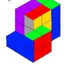
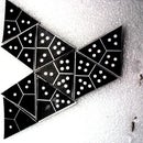
Step 11: MORE EXAMPLES

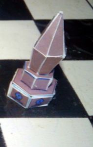
The images above show a set of patterns for making a chess piece, a Black Bishop using 2-D cardboard shapes to construct a 3-D model. The model is shown in two forms, one with hexagonal prism geometry and the other with cylindrical & conical geometry.

Anyone interested in constructing more complex objects from cardboard or sheet metal should download a copy of " Sheet Metal Drafting" by E.M.Longfield (1921) from

https://ia800206.us.archive.org/8/items/sheetmetal...

Although the author mainly describes engineering drawing methods for producing development patterns, the methods can easily be adapted to solutions based on solid geometry and graph plotting as described above. The sections titled "Related Mathematics" in the book give much useful information, although his use of fractional Imperial measurements is a little off-putting for anyone who is used to working in metric !