Graphing With Processing

Back at it again with part 2 of the plate and ball project!

If you haven't checked it out, last time I hooked up a 5-wire resistive touch screen to a DP32 and got it to read and send XY coordinate pairs through Serial.

This time I'm working on graphing those points in Processing so we can see what the DP32 is seeing.

Let's get started!

~~~~~~~~

This is part 2 of the plate and ball project. I'm trying to emulate 271828-'s Plate and Ball project using my own stuff, and I'm taking you along with me! This project will eventually cover everything from sensors to control theory, and will be a learning process for both of us! I'm very excited.

Part 1.

Step 1: Why Am I Doing This?

Visualizing data as soon as possible is very important when dealing with sensors. While playing around with this project earlier this year, I painstakingly collected and graphed over a thousand data points from this very touch-panel. What I got was the graph above.

As you can see, it bows in the middle and some of the points aren't perfectly aligned with the rest. If I want to get precise and reliable data from this sensor, I need to get rid of that bowing and filter out some noise.

However, the process of getting that graph was grueling, and the more difficult it is for a human to take data, the more chance there is for error. This project is going to be the first step in getting good, clean data, and making it easy to collect!

Step 2: What You'll Need

Because we're starting off on the tail for the previous project, you'll need everything from that one:

• 5-wire touch screen.
• Microcontroller. I'm using my trusty DP32.
• Assorted cables and connectors.
• Devil Duck is optional, but useful.

In addition, you're going to need the Processing IDE.

Step 3: Installing Grafica

This project revolves around a graphing library called Grafica.

To install it, you'll want to go to the Sketch menu:

Sketch > Import Library > Add Library

That'll open a window where you can search for Grafica*. Once you've found it, you can hit the "install" button in the lower right corner.

* I commonly misspell it as "graphica" which... won't work.

Step 4: Software Development

Now it's time to start programming.

As you can see, my program doesn't do much to start, but I'm going to take you with me as I develop something functional.

Step 5: Locating the Port

First off, we've gotta get our Processing program to start talking to the microcontroller. To do this, we import the Serial library. That'll be in Sketch > Import Library > Serial.

This will stick a line of code up at the top of your program, so I move it down into the Libraries section of my code.

Next, add the line:

printArray(Serial.list());

This line will simply list all the serial ports currently available to the program.

In picture 3, you can see a list of serial ports in the terminal (at the bottom). One of these ports should look familiar. When programming our microcontroller, we're asked to choose a port to program to, and we'll want to pick that same port here. In my case, that's port 1.

Step 6: Reading the Port

Here you can see that I've relocated the import serial line to my libraries section. You can also see that I've added a section for variables and objects, and created a serial object (myPort) and a string (inBuffer).

In picture two, you can see how I assign myPort to port 1. That's the port I identified in the previous step. At the bottom, you can see two coordinate pairs. When I pressed the button on the DP32, it sent these coordinate pairs through Serial, to my Processing sketch!

Step 7: Tokenize the Coordinates

Right now our coordinate pairs are tied up into a single string. In order to use them, we need to pull them apart. This is called tokenization, and we have a handy function that will take care of that for us!

In the first picture, you can see that I've added a section called "Data", where I create an array of strings called "token", as well as some integers: i, x, and y*.

In the second picture, I use the splitTokens() function to split the "inBuffer" string into an array of strings. This array is stored in "tokens".

Then I use my integer i to step through each of my tokens in a for loop. I print each one to terminal, and you can see that down below!

*Don't worry about x and y for now. We'll use those in the next step.

Step 8: Convert to Integer

Even now that we've split our data string apart, it's still in a string format and we need integers. Thankfully we have a convenient function for that built into the Integer class.

You can see that I've used "Integer.parseInt()" to parse the strings in "token" into integers x and y. After that I print them (with dashes instead of triangle brackets) just to make sure everything worked right.

Step 9: Graph the Data

We've connected to our board, we've transferred a string, split it apart, and converted it into a pair of integers. Now it's finally time to import Grafica and graph that data!

To start off with, I add Grafica to my sketch by going to Sketch > Import Library > grafica. That'll add it to the top of my sketch (like in picture 2). I immediately move that down to the "Libraries" section of my sketch, and while I'm there I add a "Graph" section and create a GPlot object called plot1.

In the "Setup" function, I start by changing the size of my window to 350 pixels square. I'm going to make my plot 250 pixels square, and Graphica adds 100 pixels onto that, making for a 350 pixel window. After that, I add a "Set Up Plot" section, with all the code you see there. I've commented out some lines of code because, while they're useful we don't need to add the graph title or axies labels right now.

Going down to the "Draw" function, I add one line right below where I print my x and y integers to terminal. This simple line adds these points to my plot1 object, and grafica takes care of everything else! I don't need to muck with bounds for the graph or anything!

Below that, in its own section, I simply call each function to re-draw and update the graph.

You can see my graphed data in the last picture. Once you try it out for yourself, I think you'll be floored by grafica's power. While I was drawing this, the graph automatically printed my data, and re-sized to fit it! I didn't have to do anything!

Step 10: Format the Data and Clean Up

While the default graph format does look cool, I'm going to need something a little more readable. I also don't need all that text in the terminal, so we're going to do a little formatting to the graph, and get rid of all the "print()" commands.

First thing I do is get rid of the "i" variable. It's only used in a for-loop that we'll be deleting later.

Inside the Setup function, you can see that I've made my graph much larger: 600 by 600. The window gets enlarged to 700 square as well.

Only two lines are needed for the formatting I want. One turns the points black (0, 0, 0) and full opacity (255), while the other makes them very small, only 2 pixels in diameter.

Finally, in the Draw function, you can see that I've gotten rid of the for-loop, and all the "print()" and "println()" functions, save for three. These three simply print the x and y coordinates, separated by a tab. I've kept that in there so I have some source for the raw data that's being transferred.

You can see the final product as well. Less visually interesting, to be sure, but far more useful for my purposes.

Step 11: More Examples

And that's it! If you've followed along, you'll have learned a powerful tool for creating useful visuals very quickly.

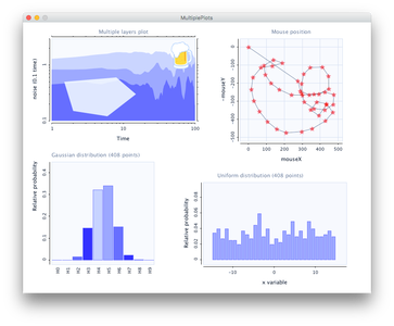
While Grafica doesn't have much in the way of documentation (that I have found) it does have quite a few examples built into the library that are useful for discovering more features and functions. These examples can be found in File > Examples, under the "Grafica" folder.

I encourage you to load them up and run them, no prep necessary. I was able to find the point color formatting function in the "ExponentialTrend" sketch, and point size formatting in the "LifeExpectancy" sketch.

I hope you found this useful, and I'll see you next time!