Introduction: Stabilize Sensor Readings With Kalman Filter
We are using various kinds of electronic sensors for our projects day to day. IMU, Ultrasonic Distance Sensor, Infrared Sensor, Light Sensor are some of them.
Most of the times we have to use a processing unit such as an Arduino board, a microcontroller chip to process the sensor data and get corresponding outputs. If we observe these readings we can identify that those are not very stable and contains noise. If we use these noisy and unstable readings for calculations and outputs, they also might contain errors. For robots, unstable and noisy readings are not suitable as they will not work well or will not do the desired task.
Therefore, we have to filter the noise and stabilize the readings of every sensor before using it for applications.
In my case, I was trying to build a Quadcopter using an Arduino 101 board and I found that the readings of the IMU are not stable. This is not good when designing a control system to stabilize the Quadcopter. Therefore, I had to find a method to filter these readings.
The mathematical model of the filter implemented here can be found on theProbabilistic Robotics by Sebastian Thrun.
Step 1: Raw Readings
First, we look at how actually noisy sensor readings look like. For this, I'm using "Pitch" values calculated by the IMU readings of the Arduino 101 board.
According to the code, the raw readings are displayed on the Serial Monitor directly. To plot these readings to visualize the noise clearly, I'm using the Serial Plotter which can found in Arduino IDE.
As you can see there are lots of spikes in the graph even the IMU is at a stable position. To avoid this we have to use a filter. Currently, there are many filter algorithms available but for my task, I have chosen the Kalman filter according to its characteristics.
Step 2: Introduction to Kalman Filter
The Kalman filter is widely used in present robotics such as guidance, navigation, and control of vehicles, particularly aircraft and spacecraft. This is essential for motion planning and controlling of field robotics, and also for trajectory optimization. Further, this is used for modeling the control of movements of central nervous systems.
The algorithm works in a two-step process.
1) Prediction
2) Estimation
In the prediction step, the filter produces estimates of the current state, along with their error probabilities. At the start, initial conditions are used. Once the next raw sensor reading is entered to the filter, these estimates are updated using a weighted average of the raw readings, with more weight being given to estimates with higher certainty.
Step 3: Filter Model
In the first image, we have the equation of the filter model. "k" represents the present state and "k-1" represents the previous state.
Let's break down the equation and try to understand it.
X(k) - Current Position
X(k-1) - Previous Position
Assume you know the previous position of an object, its velocity, and the acceleration. Then you can calculate the position of that object after a known time using the following equation.
S = ut + 0.5at^2
Here, we use the same method to estimate the current position. u(k) represents the previous velocity and the acceleration as a matrix. B(k) represents the directions of them. F(k) represents the orientation. Using these data, we can estimate the current position.
w(k) is used to indicate the unknown forces such as wind and friction.
Step 4: Basic Explanation
After estimating the current position by the previous equation, now it's compared with the actual sensor data to get the optimum output. As a result of this, noises and errors of the raw sensor readings are removed. Basically, we can get a smooth output using a spiky input of readings.
The filter is not sensitive to sudden changes in input readings. It will take few sensor readings to change the output value. As an example, if you change the pitch by 10 degrees the filter changes its output gradually and gives the output changed by 10 degrees after taking several readings. As the processing unit is getting readings on a millisecond scale, it won't take more than 10ms to reach the desired output.
The blue line of the above image shows the raw inputs and orange line shows the filtered output.
Step 5: Implementing the Algorithm
When implementing the algorithm for the Kalman filter, there are lots of mathematics to understand. Hence, it requires more time and background knowledge I will try to explain it in a simple way.
We can define the sensor readings as a Gaussian distribution, as shown in the image. The readings are distributed according to the graph and most of the readings are equal to the mean value.
When implementing the algorithm we have to define its variance in order to achieve more stable output.
Step 6: Tuning the Filter
As shown in the first image, the raw readings are passed to the filter.
To get stable and noise free output Q_angle, Q_output, and R_measure variables are need to be adjusted. These can be found at the Kalman.h header file.
Here, I have uploaded all source code files for Arduino 101. If you are using any other IMU sensors such as MPU6050, ADXL345, you can use the same code file with just small changes according to your sensor.
After tuning the output will be like this. (Blue - Raw readings, Orange - Filtered readings)
Step 7: Applications
After using this Kalman filter to my Quadcopter, which is implemented using Arduino 101 board it is very stable.
Check the following video.
You can use this filter to implement many applications such as ground robots, distance measuring devices etc.
Hope you enjoyed this instructable.
For any help regarding this or for further assistance for your projects, contact me HERE!!!
Thank You.

Participated in the
Invention Challenge 2017

Participated in the
Explore Science Contest 2017


