Designing and Testing an Electromagnetic Braking System

Rather than being a step by step procedure to make a certain object or complete a project, this instructable documents a series of projects used to complete a minor scientific investigation. I wanted to understand how electromagnets could be used as a brake on a bicycle. I also was interested in observing the relationship between the varying voltages powering the electromagnet and the corresponding retarding force produced. Here are a few things that this instructable will cover:

• How to setup an electromagnetic brake on a bicycle
• How to use an Arduino to measure the angular velocity and acceleration of a rotating wheel
• How to make a simple voltage modulator that converts AC current from a power outlet to a lower, desired DC voltage
• How to use an H bridge with an Arduino to modulate voltage
• ANOVAs and using excel to conduct ANOVAs
• Conducting t tests in excel

Some of these specific things can be found in dedicated instructables, but here they are all applied to a specific use. So not only will this instructable detail how the tasks are completed, it will serve as an example of how they can be applied. Hopefully, this instructable will inspire the reader to use this project as a starting point for some other cool hobby projects.

Theory and Main Concept
The idea of using an electromagnet as a brake has been mainly used in large vehicles and machines. There are several main types, most of which rely on using magnetism to move a mechanical part or parts. The mechanical part can then be used to produce friction with a moving part, thereby reducing speed. However, this process is rather inefficient. Electromagnets can also be used to make frictionless brakes which is what we are interested in. Further, we are interested in reducing the rotation of a bicycle wheel and hence, angular velocity. Thus, the desired brake involves dissipating rotational energy. In theory, if a magnetic field is induced in a rotating disc, it will produce eddy currents within the disc. These currents will then oppose the rotation of the disc by dissipating kinetic energy in the form of heat (causing the temperature of the disc to increase).

To me, this concept did not seem intuitive, so I decided to test it. The magnetic field is usually generated by an electromagnet. Hence, I was interested in knowing if an electromagnet could really affect the rotation of the wheel. Also, I wanted to determine whether increasing the voltage running through the electromagnet would cause a larger retarding force. The latter test may seem obvious, but I felt it was necessary to validate the concept experimentally before making any conclusions.

Step 1: Supplies and Setup

In order to test the idea of electromagnetic braking, there needs to be an apparatus with which we can experiment. We could use a bicycle, but that would be difficult to control. Instead, a single wheel should suffice. I used a 29 inch mountain bike wheel, mounted in a simple, steel frame. I also used a vise to secure the frame. To collect data, I used an Arduino Uno R3. Some old supplies were used to manipulate the electrical current. Another Arduino R3 with an H bridge and breadboard was also used to manipulate voltage; however, that part was not absolutely necessary. For the data synthesis and collection, I used a computer running Windows 8.1, Arduino IDE 1.0.5, and Excel 2013.

Here is a list of the main supplies I used (for some, I have included a link to retailers selling the item):

• 29 inch (diameter) mountain bike wheel
• Six 20.32 cm (diameter), 1 mm thick steel discs
• Parker Skinner Valve solenoid
• Arduino Uno R3
• Terminal Strip
• Soldering Iron
• 6 inch drill press vise
• Step down transformer
• Circuit board with converter (AC to DC)
• Surge protector to act as switch
• Three 4.5 inch steel screws secured to base of three pegs equidistant from each other
• AC dimmer switch (potentiometer)
• Digital Multimeter
• Breadboard wiring
• Solderless terminals and electrical wiring

Optional:

• Duel H bridge L293D
• Breadboard

Step 2: Power Supply

A 24v DC Parker solenoid was used as the electromagnet. Because a 120v AC power outlet was to be used for the power supply, I made an apparatus to convert the AC to the desired current DC. It is composed of four main parts: a power supply, a step down transformer, a circuit board, and a terminal strip. The transformer converts 120v AC to 24v AC and is connected to the input of a circuit board recycled from an old CD player. Embedded in the circuit board is a converter which provides a DC output. I had to solder the wires from the transformer to the power input on the circuit board. I was then able to use the power output wires to relay power to the terminal strip. I used male spade connectors and then some brass brackets on the terminal strip to ensure a secure connection. Everything is secured on a polycarbonate base to avoid undesirable movement during the experiment. In the picture, 1 is the cord connected to the transformer, 2 is the transformer itself, 3 is the circuit board, and 4 is the terminal strip.

If you are not using the h bridge for voltage modulation, I would recommend using a simple rheostat. I had a power strip connected to the wall outlet which acted as a switch. I could then set the rheostat to a particular setting, record the corresponding voltage, and commence with testing.

Step 3: Optional H Bridge Addition

If you want to be able to test more voltage levels, an h bridge is a simple addition. The terminal strip can be used to relay the power to an h bridge as shown in the picture. Usually, h bridges are used with robots to control the speed and direction of simple DC motors. For our purposes, we only need the modulation part of the h bridge (actually we will be using the pwm controls on the Arduino, but the h bridge is a means by which we can apply the PWM controls to the current coming from the wall outlet). A diagram of the h bridge I used is pictured. Note that it is a duel h bridge, so we will only be using half of the pins. The pins are numbered 1-16 starting in the upper left hand corner and moving counterclockwise. Pin 1 is the enable pin which I connect to pin 9 on the Arduino. If pin 1 is LOW then the entire power flow is halted. Also, pin 1 is capable of reading a PWM signal which will be used for modulation. Pins 2 and 7 are connected to pins 3 and 2 on the Arduino, respectively. These are used to control the direction of the current which will not change for our purposes. Essentially, when one is HIGH and the other is LOW, the current flows in a fixed direction and is reversed when the pin states change. Pins 3 and 6 serve as the output and are connected to the terminal strip which, in turn, is connected to the electromagnet. Pins 4 and 5 are both connected to ground on the breadboard. Pins 9 and 16 are all connected to 5v power. Lastly, pin 8 is connected to the power supply (terminal strip). The ground of the power supply should be connected to the ground on the breadboard. In the wiring diagram, the 9v battery represents what would be the power supply connected to the terminal strip while the solenoid represents the electromagnet connected to the terminal strip. The code to use the h bridge is really simple, here is one of my sketches (the file is attached):


const int controlPin1=2;//connected to 7 on h bridge

const int controlPin2=3;//connected to 2 on h bridge

const int enable=9; //connected to 1 on h bridge

void setup() {

pinMode(controlPin1, OUTPUT);
pinMode(controlPin2, OUTPUT);
pinMode(enable, OUTPUT);
digitalWrite(controlPin1, HIGH);
digitalWrite(controlPin2, LOW);

}

void loop() {

analogWrite(enable, 220); //write a value from 0-255;

}


The value in the analog write command can be adjusted to change the resulting power supplying the electromagnet. As the value decreases, so does the voltage of the power. Be careful not to fry the h bridge though, it can only take up to 36v.

Step 4: Electromagnet

The electromagnet is the key component of this project. I used the only one available to me, which was a Parker Skinner Valve solenoid 24v DC. Just about any reasonably sized electromagnet should suffice for collecting data, but if you are interested in implementing this system on a bicycle you will, as we shall see, need a much larger electromagnet. In order for the electromagnet to function properly, there needs to be a ferromagnetic disc upon which the electromagnet can induce a magnetic field. The larger the disc the better. Once again, I used what was available. Specifically, I used six 20.32 cm (diameter), 1 mm thick steel discs (see pictures). Since the wheel already had a disc brake rotor, I was able to drill holes in the steel discs so that they could easily attach to the hub.

After the ferromagnetic disc is set, there needs to be a way to position the electromagnet. In the case that the electromagnet is a valve solenoid, the central bolt can be secured through a hole in the frame. I used nylon spacers, washers, and a nut to secure the solenoid. The bolt was wrapped in electrical tape so that it would not slide out of the solenoid. Furthermore, a hole was drilled through its center so that another, smaller bolt could secure the solenoid onto the larger bolt.

Once the solenoid is in place, the wires can be connected to the terminal strip. Make sure the bolt is as close to the disc as possible. When I did it, the bolt was about 1mm from the disc. Any closer and the magnetic force from the bolt would cause surface contact. If it gets too close, you may want to add some cardboard or paper spacers in between the hub and the brace (as seen in the photos).

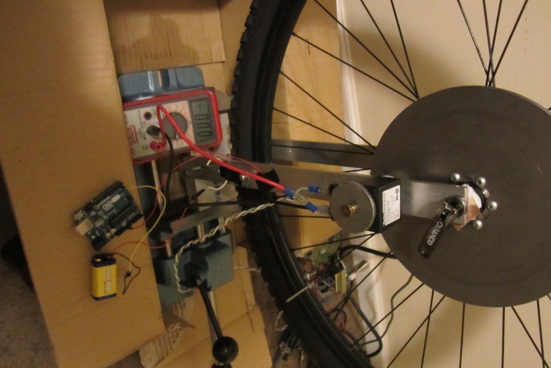
Step 5: Circuits to Collect Data

We need a method of recording the rate at which the wheel rotates and how this rate changes over time. I've employed an Arduino to record electrical impulses made by contacts around the wheel. The Arduino, connected to the computer, can then output the time intervals between the impulses which can, in turn, be graphed and analyzed appropriately.

Essentially, three screws were placed at equal distances along the rim. These served as the dynamic contact pieces of the circuit. The circuit itself consisted of a 9v battery set to the side of the wheel. The positive end of the battery was connected to a digital pin of an Arduino while the negative end was connected to a breadboard wire. The breadboard wire was secured to the aluminum stand in such a way that it would briefly make contact with a screw after one-third revolution (there would be a total of three contacts in one revolution). Another wire was secured to the aluminum part of the frame which connected to the ground of the Arduino R3 (an electrical signal was able to be transmitted from the screw to the spoke to the hub and then to the frame via the steel bearings and the steel nut attaching the hub to the aluminum frame).

With this setup, an electrical signal would be detected by the Arduino every 1/3 revolution or 2π/3 radians. Using this and the internal clock of the Arduino, the angular velocity of the wheel can be averaged for a given time interval. The results can be combined to yield an average deceleration for each trial.

Step 6: Setting Up the Arduino

Here is the program used with the Arduino (the file is attached):

const int pin=2;
unsigned long past=0;
unsigned long t=0;
unsigned long interval2=0;

void setup()
{

pinMode(pin, INPUT_PULLUP);
Serial.begin(9600);
Serial.println("Begin");

}

void loop()
{

int pin1=digitalRead(pin);

if(pin1==LOW)

{

t=millis();
interval2=t-past;
if(interval2>50)

{

Serial.println(interval2);
past=millis();
delay(10);

}

else
delay(10);

}

}

Note that this program will output the intervals in milliseconds, so we will want to take that into account for future calculations.

Step 7: Trials and Data Collection

I tested the braking system at approximately 25, 30, and 35 volts DC. Of course, the number of amperes is also important and can be combined to yield a unique watt value for each of the varying currents. They are approximately 9, 14, and 18 W, respectively (the chart summarizes this). For each level (level one being 25 volts DC etc.), I completed 15 trials. This may seem excessive, but more trials will help increase our confidence with the final results and conclusions. I also collected data of the wheel's deceleration without the solenoid. This acted as a control and served as source of comparison.

For each trial, the Arduino should be connected to the computer (if using the h bridge, a separate Arduino can be set up beforehand and powered from a different source). Make sure that the contacts are not touching the breadboard wire, initially. After uploading the program, pull up the serial monitor in the Arduino IDE (Ctrl + Shift + m). Wait for the 'begin' to output on the monitor, then give the wheel a spin. You will want to be as consistent as possible, but there will be unavoidable variation. When I was doing the trials, I tried to make sure the very first data point would be about 165 ms or in the range 180-150 ms. As soon as the wheel would begin spinning, I would turn on the power strip to begin supplying power to the solenoid. The wheel should then be allowed to freely rotate until it completely stops. As soon as the wheel stops, go to the serial monitor and copy all of the data (Ctrl + c), the paste it into a column in Excel. Do this 15 times for each voltage level.

Step 8: Data Synthesis

When collecting the raw data, the variation in the start speed of the wheel will cause variation between the data sets. To help reduce the effect of such variation, we can truncate the data to fit within a specific range. For my purposes, I discarded values outside the range [190, 1000]. To do this, I would include a simple if-then statement in the formula bar which would take the value of a certain cell and copy it if it were within the desired range and would take no action otherwise. For the first cell of the data set, this statement would look like:
=IF(AND(A1>189, A1<1001), A1, "")
This could then be extended to all the other cells in the spreadsheet.

After filtering the data, I would copy it into a new sheet. Then, I would align the columns of data according to the final recorded time interval (so that all of the final recorded time intervals were on the same row). Lastly, I would discard certain start velocities to even out all of the data sets (so that all of the first recorded time intervals would be on the same row and all of the data sets would have the same number of data points). At this point, the format of the data should resemble the format of the data in the picture above. If you were to graph one of the trials with the time interval on the y-axis against the order in which the data point was recorded on the x-axis, you should get a curve similar to the one pictured. However, we need a way to average the data from the trials so that the levels can be compared against each other.

Step 9: Converting to Angular Velocity and Average Angular Acceleration

As mentioned, it will be helpful to convert the time intervals into angular velocity and then average angular acceleration. Note that velocity is given by Δθ/Δt and that angular acceleration is given by (Δθ/Δt)/Δt. Since each impulse represents the time taken for the wheel to rotate 2π/3 radians, the average angular velocity, ω, equals 2π/3s where s is the time interval in milliseconds. To calculate the average angular acceleration, α, (deceleration in this case), we need to only consider the first and final data points. Thus, α = ((ω_f) - (ω_1)) / T where T=C - s or the cumulative total minus the first impulse and ω_f is the final angular velocity and ω_1 is the initial angular velocity (this formula is pictured above). The final result should be multiplied by 100000 to yield an answer in seconds rather than milliseconds. This formula can be applied to each cell the same way the data was filtered by the if-then statement. For the first column of a given data set in excel, this is what I would include in the formula bar:

=(((2000*PI())/(3*A84))-((2000*PI())/(3*A1)))/((SUM(A1:A84)*0.001)-A1*0.001)

This would then be applied to every other column (note that A84 is the last cell of data in my case, but it will vary from data set to data set, and A will change depending on the column). Once the average angular acceleration for each data set is calculated, the fifteen resulting values can be averaged to yield a single, all-inclusive value for that specific level. These values can be graphed as a bar graph similar to the one included. Notice the trend in the heights of the bars. This suggests that there is a direct relationship between the voltage supplied to the solenoid and the corresponding braking force; however, there is not enough evidence to draw any conclusions regarding statistical significance. Inferential statistics come in handy at this point in order to allow us to make the desired conclusions.

Step 10: ANOVA

The first step in our data analysis involves determining whether there exists a statistical difference between the data sets (that is, the probability that the difference in the data was a result of randomness). Since there are more than two data set means, an Analysis of Variance (ANOVA) test can be employed in Excel. When using this test or a t test (explained in step 12) in Excel, you do not have to worry about averaging the data beforehand. Hence, make sure all the data from the trials' average angular acceleration is located in one Excel file where you plan to complete the test. The first step is to make sure you have the Analysis ToolPak add in for Excel. If you do not (or if you are not sure), go to Excel options, Add-Ins, Analysis ToolPak, then click Go, then OK. Once you have done this, you can execute the ANOVA.

Here are the steps to execute an ANOVA:

1) Highlight all of the data
2) Click on the data tab
3) Click on Data Analysis
4) Click on ANOVA Single Factor
5) If not already selected, highlight all of the data for the input range
6) The alpha value should be set to 0.05
7) If necessary, for the output range, select a cell where you would like the results to be displayed
8) Click OK

The output should resemble the output in the picture.

There are a few important pieces of information to note with this procedure. First, the ANOVA will only compare the means of the groups. Choosing a single factor ANOVA implies that there is only one factor involved in the variation from each group mean (i.e. one independent variable; in this case, the current). Second, we are performing the ANOVA to try and reject the null hypothesis. The null hypothesis predicts that the variation in the data is a result of randomness and that there is not a distinguishable relationship between the voltage powering the electromagnet and the resulting braking force. Third, the alpha value represents the confidence level at which the test is executed. A value of 0.05 essentially means that we will be 95% confident in our conclusion. (Really it means that there is a 5% chance we will accept the null hypothesis when it is actually false or reject it when it is actually true).

Step 11: Interpreting ANOVA Results

For this study, we will focus on the f values and the p values. The f critical value represents the point which must be exceeded by the f statistic (or f ratio) in order for the null hypothesis to be rejected with 95% confidence. A large f statistic suggests that most of the variation occurs between the sets of data while a lower f statistic suggests that most of the variation occurs within the sets of data. Intuitively, if there is more variation within data sets than between data sets, it seems plausible to conclude that the null hypothesis could in fact be true. The opposite can be concluded if there is less variation within data sets than between data sets. In the case of our ANOVA pictured in step 10, the f statistic is considerably larger than the f critical value which leads us to conclude that the null hypothesis can be rejected.

The p value gives the probability that the variation between the data sets is a result of randomness. Usually, the null hypothesis can be rejected if p ≤ 0.05. In this ANOVA, the p value was extremely small, further validating our decision to reject the null hypothesis.

Step 12: T Tests

The ANOVA statistically proved the existence of nonrandom variation within the recorded data, but it did not identify the location of the variation (i.e. which data sets were statistically different; from the ANOVA we only know that there are at least two sets which are statistically different). In order to be thorough in the data analysis, it should be shown that every data set is statistically different from the other data sets. Ideally, this would be accomplished using Tukey's Post Hoc test which avoids the accumulation of errors resulting from a series of t tests, but Excel does not support this test, so we will use t tests. The error that does accumulate is negligible in this case. Here are the steps to complete a t test in excel:

1) Highlight two sets of data you would like to test
2) Go to the data tab
3) Select Data Analysis
4) Select "t-Test: Two-Sample Assuming Unequal Variances"
5) Click OK
6) For input range 1, select one of the sets of data, select the other set for range 2
7) The alpha value should be 0.05
8) If desired, choose an output area
9) Select OK

These tests should be performed with each possible combination of two data sets (i.e. control vs level 1, control vs level 2, etc.). If each p value is less than or equal to 0.05, the null hypothesis can be rejected for the totality of the project. Note that a two sample t test assuming unequal variances was used because there were two different data sets (two samples) and we do not know the variance (so we assume it is unequal).

Interpreting Results
To interpret the results, it is first necessary to understand the difference between one tail and two tailed t statistics. You can think of a normal distribution or bell curve as having two "tails" extending infinitely in both left and right directions. The one tailed t statistic considers the probability that the true population mean will exist within 5% percent of the total area under the curve in either extreme (in other words, 5% of the right tail or 5% of the left tail). The two tailed t statistic splits the 5% into 2.5% and considers both extremes (or tails) of the bell curve. By selecting the two tailed t statistic, we can increase our confidence with the conclusions. Now, consider the given t critical two tale value, denoted t_C and the actual t statistic, denoted t. If - t_C < t < t_C, then we accept the null hypothesis. In the case pictured above, the t statistic is outside this range. Therefore, we can reject the null hypothesis for these two sets of data.

Lastly, the p value is denoted "P(T<=t) two-tail" in the Excel output. Notice that in this case, p is much less than 0.05. The p values from the various tests are summarized in the table. Notice that the p values are larger for voltages close in value (i.e. level 1 and level 2, level 3 and level 2, etc.) and smaller for voltages farther in vale. This corresponds to the hypothesis that there exists a positive correlation between the voltage and the braking force produced by the electromagnet.

Step 13: Conclusion

In conclusion, the original objective was satisfied, and we know now that eddy currents can, in fact, be used with a standard bicycle wheel to produce a retarding force. Moreover, we know that with increasing voltage, the magnitude of the braking force can be increased. As follows, this system could plausibly be implemented onto a bicycle given a battery for the power supply and a sufficiently large electromagnet. There are also many other projects that could be started as continuations of this one. I will leave up to the reader to determine the next step in this instructable.

Acknowledgments:

This project couldn't have been completed without aid and advice from Geoff Koch (my dad). I am very grateful for the time he put into helping me develop an experimental design.

EDIT: I created a repository for some of this code on GitHub. It can be found here.