From Data to Graph. a Web Journey With Flask and SQLite

On my previous tutorial, Python WebServer With Flask and Raspberry Pi, we learned how to interact with the physical world, thru a web front-end page, built with Flask. So, the next natural step is collect data from the real world, having them available for us on a webpage. Very simple! But, what will happen if we want to know what was the situation on the day before, for example? Or make some kind of analyzing with those data? In those cases, we must have the data also stored in a database.

In short, on this new tutorial, we will:

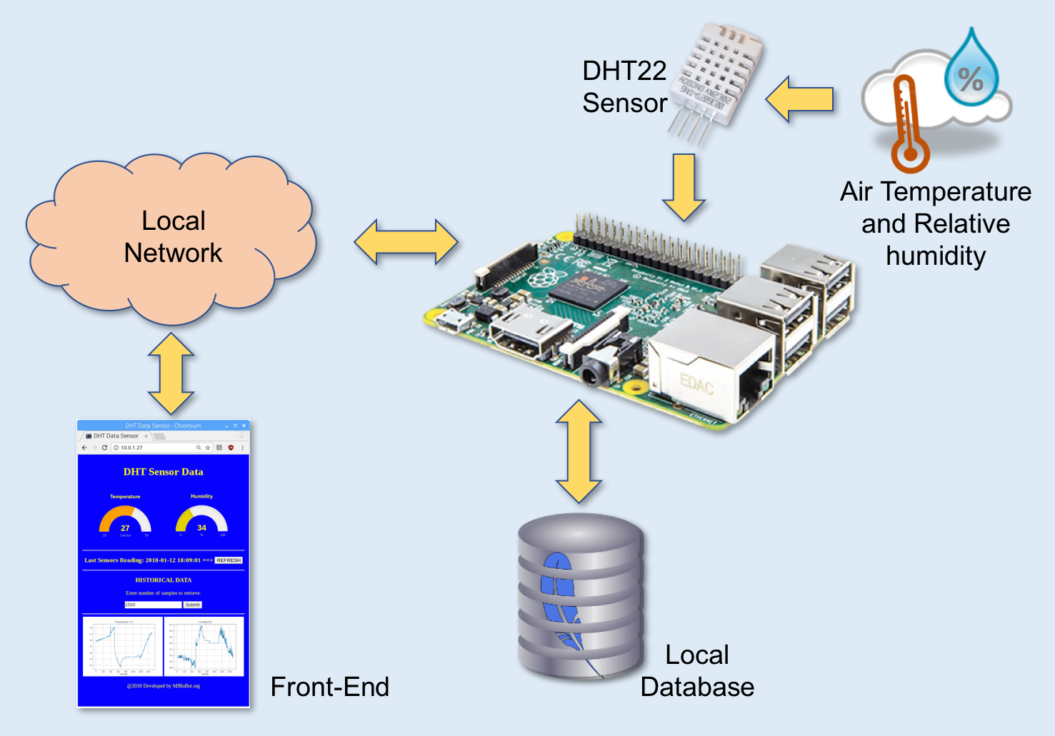
1. Capture real data (air temperature and relative humidity) using a DHT22 sensor;
2. Load those data on a local database, built with SQLite;
3. Create graphics with historical data using Matplotlib;
4. Display data with animated "gages", created with JustGage;
5. Make everything available online through a local web-server created with Python and Flask;

The block diagram gives us an idea of the whole project:

Step 1: BoM - Bill of Material

1. Raspberry Pi V3 - US$ 32.00
2. DHT22 Temperature and Relative Humidity Sensor - USD 9.95
3. Resistor 4K7 ohm

Step 2: Installing SQLite

OK, the general idea will be collect data from a sensor and store them in a database.

But what database "engine" should be used?

There are many options in the market and probably the 2 most used with Raspberry Pi and sensors are MySQL and SQLite. MySQL is very known but a little bit "heavy" for use on simple Raspberry based projects (besides it is own by Oracle!). SQLite is probably the most suitable choice. Because it is serverless, lightweight, opensource and supports most SQL code (its license is "Public Domain"). Another handy thing is that SQLite stores data in a single file which can be stored anywhere.

But, what's SQLite?

SQLite is a relational database management system contained in a C programming library. In contrast to many other database management systems, SQLite is not a client-server database engine. Rather, it is embedded into the end program.

SQLite is a popular public domain choice as embedded database software for local/client storage in application software such as web browsers. It is arguably the most widely deployed database engine, as it is used today by several widespread browsers, operating systems, and embedded systems (such as mobile phones), among others. SQLite has bindings to many programming languages like Python, the one used on our project.

(More on Wikipedia)

We will not enter into too many details here, but the full SQLite documentation can be found at this link: https://www.sqlite.org/docs.html

So, be it! Let's install SQLite on our Pi

Installation:

Follow the below steps to create a database.

1. Install SQLite to Raspberry Pi using the command:

sudo apt-get install sqlite3

2. Create a directory to develop the project:

mkdir Sensors_Database

3. Move to this directory:

cd mkdir Sensors_Database/

3. Give a name and create a database like databaseName.db (in my case "sensorsData.db"):

sqlite3 sensorsData.db

A "shell" will appear, where you can enter with SQLite commands. We will return to it later.

sqlite>

Commands starts with a ".", like “.help”, ".quit", etc.

4. Quit the shell to return to the Terminal:

sqlite> .quit

The above Terminal print screen shows what was explained.

The "sqlite>" above is only to ilustrated how the SQLite shell will appear. You do not need to type it. It will appear automatically.

Step 3: Create and Populating a Table

In order to log DHT sensor measured data on the database, we must create a table (a database can contain several tables). Our table will be named "DHT_data" and will have 3 columns, where we will log our collected data: Date and Hour (column name: timestamp), Temperature (column name: temp), and Humidity (column name: hum).

Creating a table:

To create a table, you can do it:

1. Directly on the SQLite shell, or
2. Using a Python program.

1. Using Shell:

Open the database that was created in the last step:

sqlite3 sensorsData.db

And entering with SQL statements:

sqlite> BEGIN;
sqlite> CREATE TABLE DHT_data (timestamp DATETIME,  temp NUMERIC, hum NUMERIC);
sqlite> COMMIT;

All SQL statements must end with ";". Also usually, those statements are written using capital letters. It is not mandatory, but a good practice.

2. Using Python

import sqlite3 as lite
import sys
con = lite.connect('sensorsData.db')
with con: 
    cur = con.cursor() 
    cur.execute("DROP TABLE IF EXISTS DHT_data")
    cur.execute("CREATE TABLE DHT_data(timestamp DATETIME, temp NUMERIC, hum NUMERIC)")

Open the above code from my GitHub: createTableDHT.py

run it on your Terminal:

python3 createTableDHT.py

Wherever the method used, the table should be created. You can verify it on SQLite Shell using the “.table” command. Open the database shell:

sqlite3> sensorsData.db

In the shell, once you use the .table command, the created tables names will appear (in our case will be only one: "DHT_table". Quit the shell after, using the .quit command.

sqlite> .table
DHT_data
sqlite> .quit

Inserting data on a table:

Let's input on our database 3 sets of data, where each set will have 3 components each: (timestamp, temp, and hum). The component timestamp will be real and taken from the system, using the built-in function 'now' and temp and hum are dummy data in oC and % respectively.

Note that the time is in "UTC", what is good because you don’t have to worry about issues related to daylight saving time and other matters. Should you want to output the date in localized time, just convert it to the appropriate time zone afterward.

Same way was done with table creation, you can insert data manually via SQLite shell or via Python. At the shell, you would do it, data by data using SQL statements like this (For our example, you will do it 3 times):

sqlite> INSERT INTO DHT_data VALUES(datetime('now'), 20.5, 30);

And in Python, you would do the same but at once:

import sqlite3 as lite
import sys
con = lite.connect('sensorsData.db')
with con:
    cur = con.cursor() 
    cur.execute("INSERT INTO DHT_data VALUES(datetime('now'), 20.5, 30)")
    cur.execute("INSERT INTO DHT_data VALUES(datetime('now'), 25.8, 40)")
    cur.execute("INSERT INTO DHT_data VALUES(datetime('now'), 30.3, 50)")

Open the above code from my GitHub: insertTableDHT.py

Run it on Pi Terminal:

python3 insertTableDHT.py

To confirm that the above code worked, you can check the data in the table via shell, with the SQL statement:

sqlite> SELECT * FROM DHT_DATA;

The above Terminal print screen shows how the table'rows will appear.

Step 4: Inserting and Verifying Data With Python

For starting, let's do the same we did before (input and retrieve data), but doing both with python and also printing the data on terminal:

import sqlite3
import sys
conn=sqlite3.connect('sensorsData.db')
curs=conn.cursor()

# function to insert data on a table
def add_data (temp, hum):
    curs.execute("INSERT INTO DHT_data values(datetime('now'), (?), (?))", (temp, hum))
    conn.commit()

# call the function to insert data
add_data (20.5, 30)
add_data (25.8, 40)
add_data (30.3, 50)

# print database content
print ("\nEntire database contents:\n")
for row in curs.execute("SELECT * FROM DHT_data"):
    print (row)

# close the database after use
conn.close()

Open the above code from my GitHub: insertDataTableDHT.py
and run it on your Terminal:

python3 insertDataTableDHT.py

The above Terminal print screen shows the result.

Step 5: DHT22 Temperature and Humidity Sensor

So far we have created a table in our database, where we will save all data that a sensor will read. We have also entered with some dummy data there. Now it is time to use real data to be saved in our table, air temperature and relative humidity. For that, we will use the old and good DHTxx (DHT11 or DHT22). The ADAFRUIT site provides great information about those sensors. Bellow, some information retrieved from there:

Overview

The low-cost DHT temperature & humidity sensors are very basic and slow but are great for hobbyists who want to do some basic data logging. The DHT sensors are made of two parts, a capacitive humidity sensor, and a thermistor. There is also a very basic chip inside that does some analog to digital conversion and spits out a digital signal with the temperature and humidity. The digital signal is fairly easy to be read using any microcontroller.

DHT11 vs DHT22

We have two versions of the DHT sensor, they look a bit similar and have the same pinout, but have different characteristics. Here are the specs:

DHT11 (usually blue)

• Ultra low cost
• 3 to 5V power and I/O
• 2.5mA max current use during conversion (while requesting data)
• Good for 20-80% humidity readings with 5% accuracy
• Good for 0-50°C temperature readings ±2°C accuracy
• No more than 1 Hz sampling rate (once every second)
• Body size 15.5mm x 12mm x 5.5mm
• 4 pins with 0.1" spacing

DHT22 (usually white)

• Low cost
• 3 to 5V power and I/O
• 2.5mA max current use during conversion (while requesting data)
• Good for 0-100% humidity readings with 2-5% accuracy
• Good for -40 to 125°C temperature readings ±0.5°C accuracy
• No more than 0.5 Hz sampling rate (once every 2 seconds)
• Body size 15.1mm x 25mm x 7.7mm
• 4 pins with 0.1" spacing

As you can see, the DHT22 is a little bit more accurate and good over a slightly larger range. Both use a single digital pin and are 'sluggish' in that you can't query them more than once every second (DHT11) or two (DHT22).

Both sensors will work fine to get Indoor information to be stored in our database.

The DHTxx has 4 pins (facing the sensor, pin 1 is the most left) :

• VCC (we can connect to external 5V or to 3.3V from RPi);
• Data out;
• Not Connected
• Ground.

We will use a DHT22 in our project.

Once usually you will use the sensor on distances less than 20m, a 4K7 ohm resistor should be connected between Data and VCC pins. The DHT22 output data pin will be connected to Raspberry GPIO 16. Check above electrical diagram connecting the sensor to RPi pins as below:

1. Pin 1 - Vcc ==> 3.3V
2. Pin 2 - Data ==> GPIO 16
3. Pin 3 - Not Connect
4. Pin 4 - Gnd ==> Gnd

Do not forget to Install the 4K7 ohm resistor between Vcc and Data pins

Once the sensor is connected, we must also install its library on our RPi. We will do this in the next step.

Step 6: Installing DHT Library

On your Raspberry, starting on /home, go to /Documents

cd Documents 

Create a directory to install the library and move to there:

mkdir DHT22_Sensor
cd DHT22_Sensor

On your browser, go to Adafruit GITHub:

https://github.com/adafruit/Adafruit_Python_DHT

Download the library by clicking the download zip link to the right and unzip the archive on your Raspberry Pi recently created folder. Then go to the directory of the library (subfolder that is automatically created when you unzipped the file), and execute the command:

sudo python3 setup.py install

Open a test program (DHT22_test.py) from my GITHUB

import Adafruit_DHT
DHT22Sensor = Adafruit_DHT.DHT22
DHTpin = 16
humidity, temperature = Adafruit_DHT.read_retry(DHT22Sensor, DHTpin)

if humidity is not None and temperature is not None:
    print('Temp={0:0.1f}*C  Humidity={1:0.1f}%'.format(temperature, humidity))
else:
    print('Failed to get reading. Try again!')

Execute the program with the command:

python3 DHT22_test.py

The above Terminal print screen shows the result.

Step 7: Capturing Real Data

Now that we have both, the sensor and our database all installed and configurated, it's time to read and save real data.

For that, we will use the code:

import time
import sqlite3
import Adafruit_DHT

dbname='sensorsData.db'
sampleFreq = 2 # time in seconds

# get data from DHT sensor
def getDHTdata():	
	DHT22Sensor = Adafruit_DHT.DHT22
	DHTpin = 16
	hum, temp = Adafruit_DHT.read_retry(DHT22Sensor, DHTpin)
	
	if hum is not None and temp is not None:
		hum = round(hum)
		temp = round(temp, 1)
		logData (temp, hum)

# log sensor data on database
def logData (temp, hum):	
	conn=sqlite3.connect(dbname)
	curs=conn.cursor()
	curs.execute("INSERT INTO DHT_data values(datetime('now'), (?), (?))", (temp, hum))
	conn.commit()
	conn.close()

# display database data
def displayData():
	conn=sqlite3.connect(dbname)
	curs=conn.cursor()
	print ("\nEntire database contents:\n")
	for row in curs.execute("SELECT * FROM DHT_data"):
		print (row)
	conn.close()

# main function
def main():
	for i in range (0,3):
		getDHTdata()
		time.sleep(sampleFreq)
	displayData()

# Execute program 
main()

Open the above file from my GitHub: appDHT.py
and run it on your Terminal:

python3 appDHT.py

The function getDHTdata() captures 3 samples of DHT sensor, test them for errors and if OK, save the data on database using the function logData (temp, hum). The final part of code calls the function displayData() that prints the entire content of our table on Terminal.

The above print screen shows the result. Observe that the last 3 lines (rows) are the real data captured with this program and the 3 previous rows were the ones manually entered before.

In fact appDHT.py is not a good name. In general, "appSomething.py" is used with Python scripts on web servers as we will see further on this tutorial. But of course you can use it here.

Step 8: Capturing Data Automatically

At this point, what we must implement is a mechanism to read and insert data on our database automatically, our "Logger".

Open a new Terminal window and enter with bellow Python code:

import time
import sqlite3
import Adafruit_DHT

dbname='sensorsData.db'
sampleFreq = 1*60 # time in seconds ==> Sample each 1 min

# get data from DHT sensor
def getDHTdata():	
	DHT22Sensor = Adafruit_DHT.DHT22
	DHTpin = 16
	hum, temp = Adafruit_DHT.read_retry(DHT22Sensor, DHTpin)
	if hum is not None and temp is not None:
		hum = round(hum)
		temp = round(temp, 1)
	return temp, hum

# log sensor data on database
def logData (temp, hum):
	conn=sqlite3.connect(dbname)
	curs=conn.cursor()
	curs.execute("INSERT INTO DHT_data values(datetime('now'), (?), (?))", (temp, hum))
	conn.commit()
	conn.close()

# main function
def main():
	while True:
		temp, hum = getDHTdata()
		logData (temp, hum)
		time.sleep(sampleFreq)

# ------------ Execute program 
main()

Or get it from my GitHub: logDHT.py. Run it on the Terminal:

python3 logDHT.py

What the main() function does is:

1. Call the function getDHTdata(), that will return the captured data by the DHT22 sensor.
2. Take those data (temperature and humidity) and passing them to another function: logData(temp, hum) that insert them, together with actual date and time, to our table.
3. And goes to sleep, waiting until the next scheduled time to capture data (defined by sampleFreq, which in this example is 1 minute).

Leave the Terminal window opened.

Until you kill the program with [Ctr+z], for example, the program will continuously capture data, feeding them in our database. I left it running for a while on a frequency of 1 minute for populating the database quicker, changing the frequency after few hours to 10 minutes.

There are other mechanisms much more efficient to perform this kind of "automatic logger" than using "time.sleep", but the above code will work fine for our purpose here. Anyway, if you want to implement a better "scheduler", you can use Crontab, which is a handy UNIX tool to schedule jobs. A good explanation of what Crontab is can be found in this tutorial: "Schedule Tasks on Linux Using Crontab", by Kevin van Zonneveld.

Step 9: Queries

Now that our database is being fed automatically, we should find ways to work with all those data. We do it with queries!

What is a query?

One of the most important features of working with SQL language over databases is the ability to create "database queries". In other words, queries extract data from a database formatting them in a readable form. A query must be written in SQL language, that uses a SELECT statement to select specific data.

We have in fact use it on a "broad way" on last step: "SELECT * FROM DHT_data"

Examples:

Let's create some queries over the data on the table that we have already created. For that, enter with below code:

import sqlite3
conn=sqlite3.connect('sensorsData.db')
curs=conn.cursor()

maxTemp = 27.6

print ("\nEntire database contents:\n")
for row in curs.execute("SELECT * FROM DHT_data"):
    print (row)

print ("\nDatabase entries for a specific humidity value:\n")
for row in curs.execute("SELECT * FROM DHT_data WHERE hum='29'"):
    print (row)
    
print ("\nDatabase entries where the temperature is above 30oC:\n")
for row in curs.execute("SELECT * FROM DHT_data WHERE temp>30.0"):
    print (row)
    
print ("\nDatabase entries where the temperature is above x:\n")
for row in curs.execute("SELECT * FROM DHT_data WHERE temp>(?)", (maxTemp,)):
    print (row)

Or get it from my GitHub: queryTableDHT.py, and run it on Terminal:

python3 queryTableDHT.py

You can see the result on the Terminal's print screen above. Those are simple examples to give you an idea regarding queries. Take a time to understand the SQL statements in above code.

If you want to know more about SQL language, a good source is W3School SQL Tutorial

Step 10: Last Data Entered on a Table:

A very important query is the one to retrieve the last data entered (or logged) on a table. We can do it directly on the SQLite shell, with the command:

sqlite> SELECT * FROM DHT_data ORDER BY timestamp DESC LIMIT 1;

Or running a simple python code as below:

import sqlite3
conn = sqlite3.connect('sensorsData.db')
curs=conn.cursor()

print ("\nLast Data logged on database:\n")
for row in curs.execute("SELECT * FROM DHT_data ORDER BY timestamp DESC LIMIT 1"):
    print (row)

You can see the result on the first Terminal print screen above.

Note that the result will appear as a "tuple of values": ('timestamp', temp, hum)

The tuple returned the last row content of our table, which is formed with 3 elements on it:

• row[0] = timestamp [string]
• row[1] = temp [float]
• row[2] = hum [float]

So, we can work better our code, to retrieve “clean” data from the table, for example:

import sqlite3
conn=sqlite3.connect('sensorsData.db')
curs=conn.cursor()

print ("\nLast raw Data logged on database:\n")
for row in curs.execute("SELECT * FROM DHT_data ORDER BY timestamp DESC LIMIT 1"):
    print (str(row[0])+" ==> Temp = "+str(row[1])+"	Hum ="+str(row[2]))

Open the file from my GitHub: lastLogDataTableDHT.py and run it on Terminal:

python3 lastLogDataTableDHT.py

You can see the result on the 2nd Terminal print screen above.

Step 11: A Web Front-end for Data Visualization

On my last tutorial: Python WebServer With Flask and Raspberry Pi, we learned how to implement a web-server (using Flask) to capture data from sensors and show their status on a web page.

This is what we also want to accomplish here. The difference is in the data to be sent to our front end, that will be taken from a database and not directly from sensors as we did on that tutorial.

Creating a web-server environment:

The first thing to do is to install Flask on your Raspberry Pi. If you do not have it, go to the Terminal and enter:

sudo apt-get install python3-flask

The best when you start a new project is to create a folder where to have your files organized. For example:

from home, go to our working directory:

cd Documents/Sensors_Database

Create a new folder, for example:

mkdir dhtWebServer

The above command will create a folder named "dhtWebServer", where we will save our python scripts:

/home/pi/Documents/Sensor_Database/rpiWebServer

Now, on this folder, let's create 2 sub-folders: static for CSS and eventually JavaScript files and templates for HTML files. Go to your newer created folder:

cd dhtWebServer

And create the 2 new sub-folders:

mkdir static

and

mkdir templates

The final directory "tree", will look like:

├── Sensors_Database
       ├── sensorsData.db
       ├── logDHT.py
       ├── dhtWebSensor
               ├── templates
               └── static

We will leave our created database on /Sensor_Database directory, so you will need to connect SQLite with "../sensorsData.db"

OK! With our environment in place let's assemble the parts and create our Python WebServer Application. The above diagram gives us an idea of what should be done!

Step 12: The Python WebServer Application

Starting from the last diagram, let's create a python WebServer using Flask. I suggest Geany as the IDE to be used, once you can work simultaneously with different types of files (.py, .html and .css)

The code below is the python script to be used on our first web-server:

from flask import Flask, render_template, request
app = Flask(__name__)

import sqlite3

# Retrieve data from database
def getData():
	conn=sqlite3.connect('../sensorsData.db')
	curs=conn.cursor()

	for row in curs.execute("SELECT * FROM DHT_data ORDER BY timestamp DESC LIMIT 1"):
		time = str(row[0])
		temp = row[1]
		hum = row[2]
	conn.close()
	return time, temp, hum

# main route 
@app.route("/")
def index():	
	time, temp, hum = getData()
	templateData = {
		'time': time,
		'temp': temp,
		'hum': hum
	}
	return render_template('index.html', **templateData)

if __name__ == "__main__":
   app.run(host='0.0.0.0', port=80, debug=False)

You can get the python script appDhtWebServer.py from my GitHub

What the above code does is:

• Every time that someone "clicks"'on "/", that is the main page (index.html) of our webpage a GET request is generated;
• With this request, the first thing done in the code is to take data from the database using the function time, temp, hum = getData(). This function is basically the same query that was used before to retrieve a data stored in the table.
• With the data on hand, our script returnsto the webpage (index.html): time, temp and hum as a response to the previous request.

So, let's see the index.html and style.css files that will be used to build our front-end:

index.html

<!DOCTYPE html>
   <head>
      <title>DHT Sensor data </title>
      <link rel="stylesheet" href='../static/style.css'/>
   </head>
   <body>
	<h1>DHT Sensor Data </h1>
	<h3> TEMPERATURE   ==>  {{ tempLab  }} oC</h3>
	<h3> HUMIDITY (Rel.) ==>  {{ humLab  }} %</h3>
	<hr>
	<h3> Last Sensors Reading: {{ time }} ==> <a href="/"class="button">REFRESH</a></h3>	
	<hr>
	<p> @2018 Developed by MJRoBot.org</p>
   </body>
</html>

You can get the file index.html from my GitHub

style.css

body{
	background: blue;
	color: yellow;
	padding:1%
}

.button {
	font: bold 15px Arial;
	text-decoration: none;
	background-color: #EEEEEE;
	color: #333333;
	padding: 2px 6px 2px 6px;
	border-top: 1px solid #CCCCCC;
	border-right: 1px solid #333333;
	border-bottom: 1px solid #333333;
	border-left: 1px solid #CCCCCC;
}

You can get the file style.css from my GitHub

The files must be placed in your directory like this:

├── Sensors_Database
       ├── sensorsData.db
       ├── logDHT.py
       ├── dhtWebSensor
               ├── appDhtWebSensor.py
               ├── templates
	       │      ├── index.html
               └── static
                      ├── style.css

Now, run the python script on the Terminal:

sudo python3 appDhtWebServer.py

Go to any browser in your network and enter with http://YOUR_RPI_IP (for example, in my case: http://10.0.1.27)

The above print screen shows what you must see.

NOTE: If you are not sure about your RPi Ip address, run on your terminal:

 ifconfig

at wlan0: section you will find it. In my case: 10.0.1.27

Step 13: Making Our Web Front-End Fancier!

Let's introduce some Gages to present actual Temperature and Humidity values on a better way. Note that our Python script will not change, but using JustGage on our html/css files, will improve a lot how data will be presented.

What is JustGage?

JustGage is a handy JavaScript plugin for generating and animating nice & clean gauges. It is based on Raphaël library for vector drawing, so it’s completely resolution independent and self-adjusting, working in almost any browser.

Installation:

1. Download JustGage v1.2.2 + Examples from JustGage website ==> http://justgage.com/download/justgage-1.2.2.zip
2. Save the 2 .js files on /static/ directory
3. Use the new index.html below:

<!doctype html>
<html>

<head>
    <title>DHT Data Sensor</title>
    <link rel="stylesheet" href='../static/style.css'/>
    <meta http-equiv="Content-Type" content="text/html; charset=UTF-8" />
    <style>
	body {
	    text-align: center;
	}
	#g1,
	#g2 {
	    width: 200px;
	    height: 160px;
	    display: inline-block;
	    margin: 1em;
	}
   </style>
</head>
<body>
    <h1>DHT Sensor Data </h1>
    <div id="g1"></div>
    <div id="g2"></div>
    <hr>
	<h3> Last Sensors Reading: {{ time }} ==> <a href="/"class="button">REFRESH</a></h3>	
	<hr>
	<p> @2018 Developed by MJRoBot.org</p>
    
    <script src="../static/raphael-2.1.4.min.js"></script>
    <script src="../static/justgage.js"></script>
    <script>
	var g1, g2;
	document.addEventListener("DOMContentLoaded", function(event) {
	    g1 = new JustGage({
		id: "g1",
		value: {{temp}},
		valueFontColor: "yellow",
		min: -10,
		max: 50,
		title: "Temperature",
		label: "Celcius"
	});
	    g2 = new JustGage({
		id: "g2",
		value: {{hum}},
		valueFontColor: "yellow",
		min: 0,
		max: 100,
		title: "Humidity",
		label: "%"
	});
      });
    </script>
</body>
</html>

Download from my GitHub the file: index_gage.html, and rename it as index.html (do not forget of renaming the previous one with a different name if you want to keep it, for example, index_txt.html).

The final directory tree should like as below:

├── Sensors_Database
       ├── sensorsData.db
       ├── logDHT.py
       ├── dhtWebServer
               ├── appDhtWebServer.py
               ├── templates
	       │      ├── index.html
               └── static
                      ├── style.css
                      ├── justgage.js
		      ├── raphael-2.1.4.min.js

Press[Crl-C] on your Terminal to Quit appDhtWebServer.py and just start it again. When you refresh your browser you must see the above print screen.

Look the examples files that you downloaded from JustGage website. Try make changes on your gages. It is very simple.

Step 14: The Full Proccess

The above diagram resumes what we have accomplished so far: 2 separate scripts running in parallel, doing their tasks independently:

1. Capturing data with sensor and load them into a database (logDHT.py)
2. Look for data on the database and present them on a web front-end (appDhtWebServer.py).

In general terms our project of capture data, saving them on a database and displaying those data on a webpage is finish. But make no sense to have a database with historical data and only use it for the last data captured. We must play with historical data and the most basic thing to do is presented them on a graph. Let's go to it!

Step 15: Graphing the Historical Data

A very good library to graph data is Matplotlib, that is a Python 2D plotting library which produces publication quality figures in a variety of hardcopy formats and interactive environments across platforms.

To install matplotlib, run the command below on your Terminal:

sudo apt-get install python3-matplotlib

Before we start, let's create a new environment, where we will save the new application to be developed: appDhtWebHist.py and its correspondent index.html and style.css

├── Sensors_Database
       ├── sensorsData.db
       ├── logDHT.py
       ├── dhtWebHist
               ├── appDhtWebHist.py
               ├── templates
	       │      ├── index.html
               └── static
                      ├── style.css

Create the new 3 directories (dhtWebHist; /templates and /static) same as we did before and open from my GitHub the 3 files below:

1. appDhtWebHist.py

from matplotlib.backends.backend_agg import FigureCanvasAgg as FigureCanvas
from matplotlib.figure import Figure
import io

from flask import Flask, render_template, send_file, make_response, request
app = Flask(__name__)

import sqlite3
conn=sqlite3.connect('../sensorsData.db')
curs=conn.cursor()

# Retrieve LAST data from database
def getLastData():
	for row in curs.execute("SELECT * FROM DHT_data ORDER BY timestamp DESC LIMIT 1"):
		time = str(row[0])
		temp = row[1]
		hum = row[2]
	#conn.close()
	return time, temp, hum

def getHistData (numSamples):
	curs.execute("SELECT * FROM DHT_data ORDER BY timestamp DESC LIMIT "+str(numSamples))
	data = curs.fetchall()
	dates = []
	temps = []
	hums = []
	for row in reversed(data):
		dates.append(row[0])
		temps.append(row[1])
		hums.append(row[2])
	return dates, temps, hums

def maxRowsTable():
	for row in curs.execute("select COUNT(temp) from  DHT_data"):
		maxNumberRows=row[0]
	return maxNumberRows

# define and initialize global variables
global numSamples
numSamples = maxRowsTable()
	if (numSamples > 101):
numSamples = 100

# main route
@app.route("/")
def index():
	time, temp, hum = getLastData()
	templateData = {
	  	'time'	: time,
		'temp'	: temp,
      		'hum'	: hum,
      		'numSamples'	: numSamples
	}
	return render_template('index.html', **templateData)

@app.route('/', methods=['POST'])
def my_form_post():
    global numSamples
    numSamples = int (request.form['numSamples'])
    numMaxSamples = maxRowsTable()
    if (numSamples > numMaxSamples):
        numSamples = (numMaxSamples-1)
    time, temp, hum = getLastData()
    templateData = {
	  	'time'	: time,
      		'temp'	: temp,
      		'hum'	: hum,
      		'numSamples'	: numSamples
	}
    return render_template('index.html', **templateData)

@app.route('/plot/temp')
def plot_temp():
	times, temps, hums = getHistData(numSamples)
	ys = temps
	fig = Figure()
	axis = fig.add_subplot(1, 1, 1)
	axis.set_title("Temperature [°C]")
	axis.set_xlabel("Samples")
	axis.grid(True)
	xs = range(numSamples)
	axis.plot(xs, ys)
	canvas = FigureCanvas(fig)
	output = io.BytesIO()
	canvas.print_png(output)
	response = make_response(output.getvalue())
	response.mimetype = 'image/png'
	return response

@app.route('/plot/hum')
def plot_hum():
	times, temps, hums = getHistData(numSamples)
	ys = hums
	fig = Figure()
	axis = fig.add_subplot(1, 1, 1)
	axis.set_title("Humidity [%]")
	axis.set_xlabel("Samples")
	axis.grid(True)
	xs = range(numSamples)
	axis.plot(xs, ys)
	canvas = FigureCanvas(fig)
	output = io.BytesIO()
	canvas.print_png(output)
	response = make_response(output.getvalue())
	response.mimetype = 'image/png'
	return response

if __name__ == "__main__":
   app.run(host='0.0.0.0', port=80, debug=False)

A new function was created here: getHistData (numSamples), that receives as a parameter the number of rows that should be taken from the database. Basically, it is very similar to getLastData(), where numSamples was "1". Of course, now we must "append" the return array for all required rows.

In fact, we could use only this last function for both tasks.

The number of samples is set by default as 100, at the beginning (if there are more them 100 rows into the database) and also received it as an input from the webpage, during normal operation. When we receive the number of samples to be retrieved, we must also check if it is lower than the maximum number of rows in the database (otherwise we will get an error). The function maxRowsTable(), returns this number.

With the historical data in hand: times, temps and hums that are arrays, we must build the graphs saving them as a .png ímage. Those images will be the return for the routes:

• @app.route('/plot/temp') and
• @app.route('/plot/hum').

The request for the images is done by index.html, by the IMG TAG.

2. index.html

<!DOCTYPE html>
   <head>
      <title>DHT Sensor data </title>
      <link rel="stylesheet" href='../static/style.css'/>
   </head>
   <body>
	<h1>DHT Sensor Data </h1>
	<h3> TEMPERATURE   ==>  {{ temp  }} oC</h3>
	<h3> HUMIDITY (Rel.) ==>  {{ hum  }} %</h3>
	<hr>	
	<h3> Last Sensors Reading: {{ time }} ==> <a href="/"class="button">REFRESH</a></h3>	
	<hr>
	<h3> HISTORICAL DATA </h3>
	<p> Enter number of samples to retrieve:
	<form method="POST">
		<input name="numSamples" value= {{numSamples}}>
		<input type="submit">
		</form></p>
	<hr>
	<img src="/plot/temp" alt="Image Placeholder" width="49%">
	<img src="/plot/hum" alt="Image Placeholder" width="49%">
	<p> @2018 Developed by MJRoBot.org</p>
   </body>
</html>

3. style.css

body{
	background: blue;
	color: yellow;
	padding:1%
}

.button {
	font: bold 15px Arial;
	text-decoration: none;
	background-color: #EEEEEE;
	color: #333333;
	padding: 2px 6px 2px 6px;
	border-top: 1px solid #CCCCCC;
	border-right: 1px solid #333333;
	border-bottom: 1px solid #333333;
	border-left: 1px solid #CCCCCC;
}

img{
	display: display: inline-block
}

The above print screen shows the result.

Step 16: Including Gage on History Webpage

If instead of text, you want also to include gages to display the actual data, you must have the 2 .js files that you have used before on /static subdirectory and change the index.html file on /templates:

Below how the directory tree looks like:

├── Sensors_Database
       ├── sensorsData.db
       ├── logDHT.py
       ├── dhtWebHist
               ├── appDhtWebHist.py
               ├── templates
	       │      ├── index.html
               └── static
                      ├── style.css
                      ├── justgage.js
		      ├── raphael-2.1.4.min.js

From my GitHub, open index_gage.html and rename it index.html. Replace the actual index.html (text version) and voilá! You will get a beautiful webpage, showing as gages the last captured data of temperature and humidity by the DHT22 and the historical graphs of those data.

Press[Crl-C] on your Terminal to Quit appDhtWebServer.py and just start it again. When you refresh your browser you must see the above print screen.

Step 17: Retrieving Data by Time Instead of Samples

So far we have build our gphics based on historical data, sending as a input parameter the numbers of samples to be retrieved from our database. Alternativelly we could use as a paramater the number of past minutes that we want to show on a graph.

In order to do that, the first thing to know is the frequency of logged data on our database. Remember that this task is done for an independent program (in our case, logDHT.py). One simple way to finfd this frequency is to retrieve the last 2 data logged on database and subtracting their correspondent timeStamp data:

in general terms: frequency = timeStamp(1) - timeStamp(0)

The function below does the work for us, using "datetime.striptime()":

# Get sample frequency in minutes
def freqSample():
	times, temps, hums = getHistData (2)
	fmt = '%Y-%m-%d %H:%M:%S'
	tstamp0 = datetime.strptime(times[0], fmt)
	tstamp1 = datetime.strptime(times[1], fmt)
	freq = tstamp1-tstamp0
	freq = int(round(freq.total_seconds()/60))
	return (freq)

Once we we have this frequency paramater in minutes, we will show it on index.html and asking for a "rangeTime" number of minutes to be send back to our server ==> @app.route('/', methods=['POST']):

@app.route('/', methods=['POST'])
def my_form_post():
    global numSamples 
    global freqSamples
    global rangeTime
    rangeTime = int (request.form['rangeTime'])
    if (rangeTime < freqSamples):
        rangeTime = freqSamples + 1
    numSamples = rangeTime//freqSamples
    numMaxSamples = maxRowsTable()
    if (numSamples > numMaxSamples):
        numSamples = (numMaxSamples-1)

The above picture shows the result.

Eliminating Possible errors when constructing the graphs:

Ocasionally, strange (or corrupted) data can be storaged on database, jeopardizing our analysis. Those data can be verified (or cleaneed) on several places (like during the time sensor are capturing the data, etc). But once the script that display data is independent of the one that logged the data, let's "cap" the maximum and minimum values of our sensors, before using the data to buit the graphs. This can be achieved with the function testData(temps, hums):

# Test data for cleanning possible "out of range" values
def testeData(temps, hums):
	n = len(temps)
	for i in range(0, n-1):
		if (temps[i] < -10 or temps[i] >50):
			temps[i] = temps[i-2]
		if (hums[i] < 0 or hums[i] >100):
			hums[i] = temps[i-2]
	return temps, hums

The scripts for this new version can be download from my GitHub: dhtWebHist_v2

Step 18: Conclusion

As always, I hope this project can help others find their way into the exciting world of electronics!

For details and final code, please visit my GitHub depository: RPI-Flask-SQLite

For more projects, please visit my blog: MJRoBot.org

Saludos from the south of the world!

See you at my next instructable!

Thank you,

Marcelo