How to Create and Label a Pie Chart in Excel 2013

The purpose of this step-by-step guide is to explain the process of creating and labeling a pie chart in Excel 2013. A pie chart is a circular statistical graphic which is divided into slices to illustrate numerical proportion. They are widely used in business as well as other areas and, chances are, you're going to need to create one at some point in your career. Pie charts have a multitude of advantages, such as:

· Displaying relative proportions of multiple classes of data

· Summarizing a large data set in visual form

· Being visually simpler than other types of graphs

What you're going to need: a computer or laptop with Microsoft Excel 2013 installed on it.

Step 1: Getting Started

Open Microsoft Excel 2013 and click on the “Blank workbook” option.

Step 2: Input the Data

Create your spreadsheet by inputting the numbers and labels which are going to be used in the pie chart. In this example, I used the labels “Desserts”, “Appertizers”, “Entrees”, “Beer”, and “Wine”.

Step 3: Select the Cells

Highlight the numbers and labels which are going to be used in the pie chart by left-clicking on a cell and then dragging the cursor across the other cells.

Step 4: Locate and Click "Insert"

Click the “Insert” menu from the toolbar located at the top of the spreadsheet. This will give you access to the "Charts" group.

Step 5: Click on the Icon

Under the “Charts” group,click on the mini pie chart icon and then a drop-down menu with available pie charts will appear.

Step 6: Choose a Pie Chart

Click on your preferred pie chart and it will appear in the middle of your spreadsheet. In this example, I used a 3-D pie chart.

Note: You can re-position the pie chart by left-clicking it and dragging it to your preferred position.

Step 7: Click on the First Box

Click on the pie chart that appeared on your screen, and then, out of the 3 boxes that will appear on its right side, click on the cross.

Step 8: Label the Chart

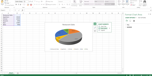
Check the “Data Labels” square and the labels will appear on the pie chart. Congratulations, you have successfully created a labeled pie chart.

Note: If you want to re-position the labels, hover your cursor over the “Data Labels” option and click on the small, black triangle that appears next to it. A drop-down menu will appear with different label positions.