This Instructable will demonstrate the steps that it takes to do change of variables in Cartesian double integrals. It is important that readers understand that there is knowledge that is required before viewing this Instructable.

Before viewing, readers should understand the following:

-In depth concepts of an introductory Calculus class
-Concepts and nature of multi-variable functions
-What double integrals are and how to evaluate them
-Cartesian and Polar 2D coordinate systems

These instructions will work through change of variables for a particular integral but they can be applied for nearly any double integral.

Step 1: Choose Your Substitutions

These instructions will work through the double integral above over the given region. The first step is to choose the substitutions that we want to use. Clearly, the integral the way it is given is not the easiest to evaluate. The whole point in choosing substitutions is to make the integral easier. Also, we will need to make as many substitutions as there are variables in the integral. In our case this means we need to make 2 substitutions. Typically u and v are used. With the given integral it would be much easier if we chose u = x + y and v = x - y.

Step 2: Solve the Substitutions for X and Y

The substitutions that we just chose should be a U expressed with X's and Y's and a V expressed with X's and Y's. The next step is to solve them for X expressed with U's and V's and Y expressed with U's and V's. With an arbitrary integral with n variables, the substitutions will form a nxn system of equations that will need to be solved for the starting variables. In our case the substitutions form a 2x2 system of equations that we can solve for X and Y. If we do so we get X = (u +v)/2 and Y = (v - u)/2.

Step 3: Find the Jacobian Determinant

The Jacobian is a determinant of a matrix that involves X differentiated with respect to U and V as well as Y differentiated with respect to U and V. For an integral with n variables, there will be n substitutions and the Jacobian will be a nxn determinant. This is one reason that previous knowledge is required. Multivariable functions, partial derivatives, and matrix determinants are all used in this step. In our case dx/du = 1/2, dx/dv = 1/2, dy/du = -1/2, and dy/dv = 1/2. So the Jacobian Determinant is 1/2.

Step 4: Change the Differential

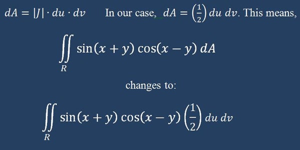
When converting double integrals to polar coordinates, we change the differential dA using the formula dA = rdrdθ. For a general change of variables we do not have a formula for the differential so we need to create one. In any change of variables, the new differential is the absolute value of the Jacobian Determinant times the differentials of the new substitution variables. So in our case, we use dA = (1/2)dudv.

Step 5: Change the Function

This step is arguably the easiest step in the whole process. We chose our substitutions so that the integral would become easier. All we have to do now is take the substitutions we made and plug them into the function. The end result should be a function of U's and V's. It should also look much simpler and easier to integrate then the original function.

Step 6: Draw the X-Y Region

This and the next few steps are geared towards changing the region of integration. We eventually want to figure out bounds for our substitution variables U and V. In order to do this it is going to be most helpful to first draw the initial region of integration. Note that the dimension of the region of integration is equal to the number of integrals in the problem. This means it is not possible to draw the original region in a quadruple integral or more. In these cases a more mathematical analysis of the region is required.

Step 7: Draw the X-Y Region in the U-V Plane

The next step is to take our region and sketch it on a U-V grid. Since our region is given by vertices that are Cartesian coordinate points, all we have to do is convert the X-Y points to U-V points. To do this we will again use our initial substitutions. For the origin, when x is 0 and y is 0, u is 0 and v is 0. So (0,0) in X-Y maps to (0,0) in U-V. When x and y are 2, u is 4 and v is 0. So (2,2) in X-Y maps to (4,0) in U-V. Also (2,-2) maps to (0,4) in U-V. We now have our region in U-V. The region is again a triangle. Note, if the initial region is given in terms of functions, the U-V region is a little harder but can be drawn.

Step 8: Set Up the Integral

We are now able to set up the final integral. With our U-V region drawn we can see that u goes from 0 to 4 and v goes from 0 to 4 minus u. All we have to do is put these bounds for U and V in the bounds of the double integral. With multiple integrals there are some key rules to follow. The outside bounds must be constant. Also, the outside bounds correspond to the outside differential and the inside bounds correspond to the inside differential. This leaves one possible way to set up the integral.

Step 9: Evaluate the Inner Integral

Now we have the integral completely set up, all that is left to do is evaluate it. In order to evaluate our specific double integral, we need to evaluate the inner one first. This requires knowledge of techniques of integration. We must first find the anti-derivative of the function with respect to V. Next we must evaluate the anti-derivative at V's upperbound and subtract what we get when we evaluate it at V's lowerbound.

Step 10: Evaluate the Final Integral

The last step is to finish evaluating the integral. The integral above did get somewhat messy. This is only because the region of integration was changed. The original region of integration was a similar triangle with vertices at (0,0), (π,π), and (π, -π). This would have made dealing with the trigonometry much easier!