Introduction: How to Create Your Own Topographic Map


When you enjoy outdoors, sometimes you are in situations where you can't find any printed topographic map that fits your plans.
There are numerous situations where you wish you knew how to create a map:
- in some countries (like Mexico) printed map are not commonly available
- when you are exploring a region that is not commonly travelled and editors doesn't bother creating maps for it
- when you don't want to bring a large map and prefer small/handy formats
- when you like to have a GPS trace or coordinates already placed on your map
- ...
In this ible I propose you to learn how to create your own topographic map and print it at home!
Supplies
- A computer
- A color printer
Beware! It takes time and practice!
Step 1: Online Tools - Offline Tools
If the personalized map you are wanting to create is located in the US there are plenty of websites that allow you to edit your own map. I personally like https://caltopo.com which is straightforward and easy to use.
If you can't find any online tool that fits your need then you'll have to create your map from scratch. In the following steps I'll show how to create such map using the software QGIS.
Step 2: Setup
- Install git on your computer: https://git-scm.com/book/en/v2/Getting-Started-In...
- Download my source repository by running the command line:
git clone --recurse-submodules -j8 https://github.com/ClemRz/Topographic-Maps.git
- Download and install the latest QGIS LTS version: https://qgis.org/en/site/forusers/download.html
- Create a free account under https://earthexplorer.usgs.gov/
Step 3: Create a Map From an Existing Map
Here is a general overview of the steps to follow:
- Open an existing map, the more recent the better
- Save it as new in a different folder under the same root directory
- Fetch the layers for your map (see next step)
- Style the layers (see step "Style layers")
- Configure the atlas layer (see step "Configure an atlas")
- Edit the print composer (see step "Compose")
- Print the map (see step "Print")
Step 4: Add Layers

Layers in a map refers to categories of visual elements in a digital form.
For instance the streets are vectors with properties attached to them: name of the street, maybe length etc. A street layer is actually a database containing all the streets and their properties.
Depending on your map's location you will fetch the layer from different services.
- For USA I use to download them from OSM, (see a how to: https://gist.github.com/ClemRz/fb09b34a6dca21dd63dbe4dd83e26634).
- For Mexico I use to download them from INEGI. The steps are (see this screencast: https://www.screencast.com/t/Uslper7CMm):
- Visualize the file named `claves_INEGI.kmz` located in `Topographic-Maps` with Google Earth for instance
- Click on the cell(s) corresponding to your area of interest. A key will be shown, for instance `A11B22`
- Go to https://www.inegi.org.mx/app/mapas/ search using the previous key and download the latest `SHP` package
- Unzip the downloaded file, move the folder to your map's folder, then drag and drop the SHP files to your QGIS map
- Download the DEM files. DEM is for Data Elevation Model, this is the source file that we will use to generate the contour lines (elevation curves) and the hill-shades (see step "DEM")
- Download any trail related file that could enrich your map, it can be a KML/KMZ file from a GPS device, or even a file downloaded from WikiLoc (https://www.wikiloc.com/) or AllTrails (https://gist.github.com/ClemRz/4b7b525bb4e7405b7f3937a695ded310)
- Download any layer that provides useful information to your map:
- Forest (https://gist.github.com/ClemRz/2b06ce8701607ccc83ea3149a84bfd1a)
- Protected Areas (https://www.protectedplanet.net/)
- RAN (https://sig.ran.gob.mx/sigIntroduccion.php)
- Etc.
Step 5: DEM
A topographic map is a map showing the third dimension, elevation, graphically. In order to do that we display what we call contour lines, AKA elevation curves. Here is how to do that:
- Go to https://earthexplorer.usgs.gov/ and log in with your account
- Delimit your zone of interest on the map
- Click `Data Sets >>`, unfold `Digital Elevation` and check `ASTER GLOBAL DEM`
- Click `Results >>` and download the rasters
- Drag and drop the rasters in your QGIS project
- Merge the rasters if you use more than one: `Raster` > `Miscellaneous` > `Merge...`
- Clip the merged raster according to the area of interest: `Raster` > `Extraction` > `Clipper`
- Get rid of all the rasters except the clipped one
- Extract the contour lines (see step "Contour Lines")
- Extract the hill-shades (see step "Hill Shades")
- Extract the slope-shades (see step "Slope Shades")
Step 6: Contour Lines

- Make sure the project's CRS is `EPSG:4326` (GPS)
- Open the `Contour` dialogue: `Raster` > `Extraction` > `Contour`
- Select the input file (the clipped raster)
- Specify the location of the output file (contour lines)
- Check the box `Attribute name` and change the name from `ELEV` with `elevation`
- Click ok
Step 7: Hill Shades
- Open the `DEM (Terrain models)` dialogue: `Raster` > `Analysis` > `DEM (Terrain Models)`
- Select the input file (the clipped raster)
- Specify the output file (the hill shade raster)
- Leave the `mode` to `Hillshade`
- Go to http://blogs.esri.com/esri/arcgis/2007/06/12/setting-the-z-factor-parameter-correctly/ and take note of the Z factor (in meters) that matches the mean latitude of your map
- Click on the "pen" button at the bottom right corner of the dialogue and change the value `-z 1.0` to `-z ` followed by the Z factor you took note previously
- Click `OK`
- Change the transparency (80%), brightness and contrast so the result is nice looking.
Step 8: Slope Shades
- Open the `DEM (Terrain models)` dialogue: `Raster` > `Analysis` > `DEM (Terrain Models)`
- Select the input file (the clipped raster)
- Specify the ouput file (the slope shade raster)
- Change the `mode` to `Slope`
- Go to http://blogs.esri.com/esri/arcgis/2007/06/12/setting-the-z-factor-parameter-correctly/ and take note of the Z factor (in meters) that matches the mean latitude of your map.
- Compute the inverse `s` of that value: `1/Z`. For instance if your Z factor is `0.00001036` the the inverse `s` is: `1/0.00001036` which is about `96525`
- Click on the "pen" button at the bottom right corner of the dialogue and change the value `-s 1.0` to `-s ` followed by the s factor you computed previously
- Click `OK`
- Change the transparency (80%), brightness and contrast so the result is nice looking.
Step 9: Style Layers

It is important to reorganize your layers into groups to preserve the following order:
- at the top level the "points" layers, we'll name the group `P`
- next, the "lines" layers, we'll name the group `L`
- next, the "area" layers, we'll name the group `A`
- at the bottom the rasters and other aerial images
Using the style copy/paste feature of QGIS it is easy to style the added layers with the existing ones:
- Right-click on an existing layer, `Styles` > `Copy Style`
- Right-click on the new equivalent layer, `Styles` > `Paste Style`
If there is no existing equivalent for a new layer, you will be able to find a library of stylings under the `QGIS-Properties` folder:
- Double-click on the new layer to open the properties dialogue
- At the bottom click on `Style` > `Load Style` and locate the matching style file
- Click `Open` and `OK`
Step 10: Configure an Atlas

An atlas is what will allow you decide and visualize in advance what will be printed in the end. It is basically a polygon layer that represents the sheets of paper. But that's not all, it also contains some information behind each sheets (polygons): the orientation (landscape or portrait), the scale and the id (for page numbering and ordering).
As you copied a recent project to start with, you should already have a layer named `atlas`.
- Edit this layer (pencil icon, or right-click then `toggle editing`)
- Copy-paste and move the pages over the areas of interest
- Open the attribute table (table icon, or right-click then `Open Attribute Table`)
- Renumber the column `id` according to your needs, change the scale if necessary
- Save the edits (floppy disk icon with a red pencil) then toggle the editing back
It is better for a trail map to have the sheets overlapping a bit.
You will be able to modify this layer whenever you want during the composing process. Don't worry if this is not perfect yet.
Step 11: Compose

The action of composing corresponds to put together the map (styled layers) with anything that could help reading it:
- a legend
- a scale
- a CRS (https://en.wikipedia.org/wiki/CRS) grid
- a title
- etc.
A composer is the tool that will help to arrange all this together on the page.
Go to the next step to start composing
Step 12: Map & Atlas

- Click on `Project` > `Print Composers` > `dynamic`
- On the right hand side, click on `Atlas generation` and make sure of the following:
- `Coverage layer` is set to `atlas`
- `Hidden coverage layer` is checked
- `Page name` is set to `id`
- `Sort by` is checked and set to `id`
- `Single file export when possible` is checked
- Click on the map, the area at the center of the page where it probably says "Map will be printed here"
- On the right hand side, click on `Item properties`
- Under the section `Main properties` change from `Rectangle` to `Cache`
- Make sure the section named `Controlled by atlas` is checked
- Make sure that, under this section, `fixed scale` is selected
- Click on the menu `Atlas` > `Preview Atlas`
At this point you should be abbe to navigate through the pages, with the icons or the same `Atlas` menu.
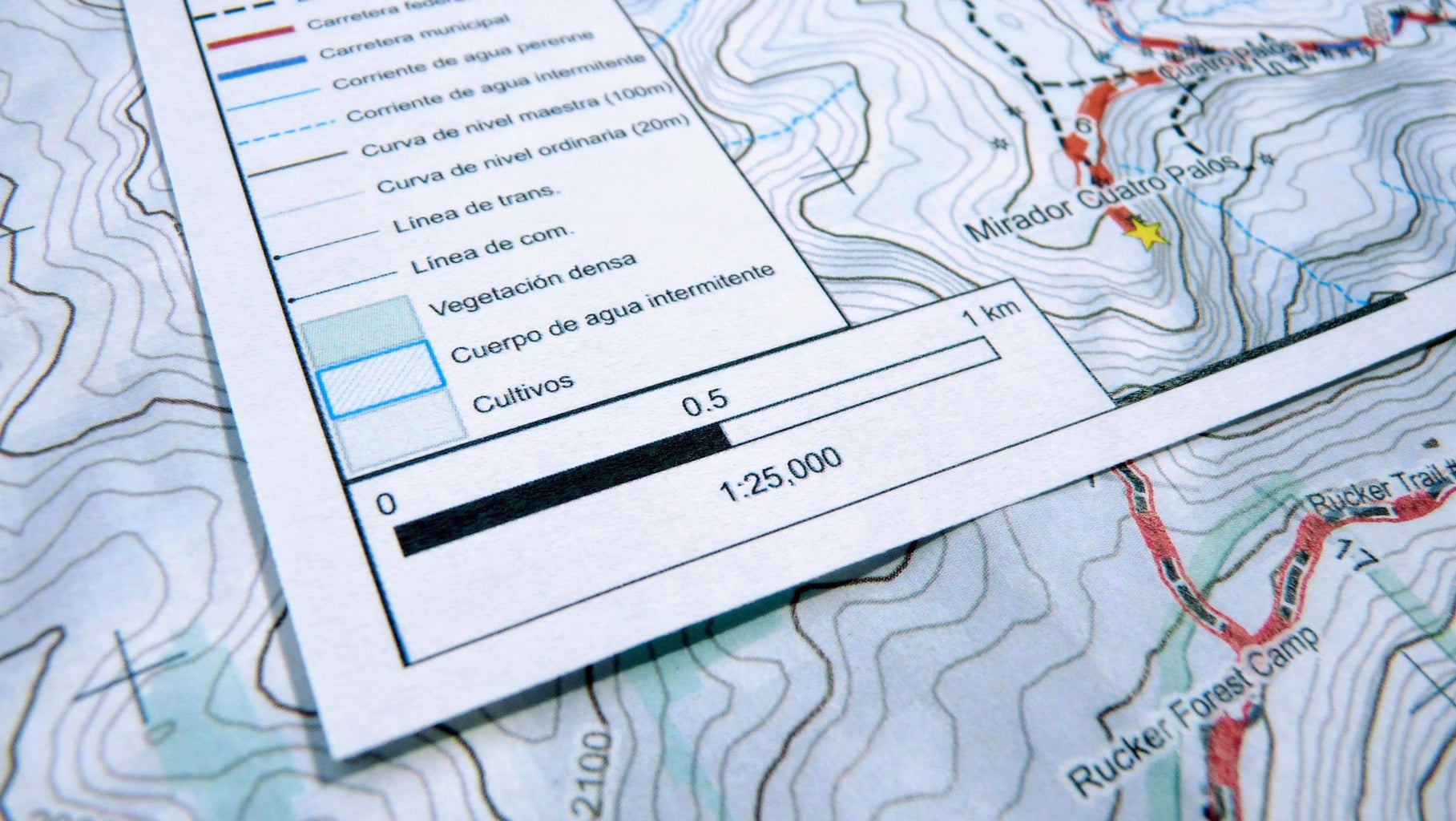
Step 13: Legend

The legend is what helps decrypt the symbology of the map.
- Click on the existing legend
- On the right hand side, click on the `Update all` button under the section `Legend items`. Make sure `Auto update` is not selected.
- You will see the same hierarchy as you grouped the layers. We don't need that hierarchy so we need to do some renaming and cleanup. Starting by dragging and dropping all the items outside of the groups so we can delete them.
- Some layer have a conditional styling, like the roads and the streams. They are easily identifiable by the arrow that appears left to the layer name. Edit that layer name (click on the pencil icon), clear the name and press `OK`.
- Remove (red `-` icon) the DEM entries such as the slope-shade, hill-shade and any layer that has no sense to be present in the legend.
- Rename the remaining entries so they make sense
Step 14: Additional Information Box

This is the text box located at the bottom right of the page. I indicates the name of the map, the number of the current page and the number of pages in total, the author, the scale, the magnetic declination etc.
- Click on the name of the map and modify it according to your needs. You will see that there are 2 placeholders for the page number and the total number of pages.
- Click on the text where appears the author and modify it according to your needs.
- Obtain the magnetic declination value for your map: go to http://twcc.fr and locate the pin where your map is. At the bottom left of the screen you will be able to read the value of the magnetic declination.
- Back in QGIS, click on the magnetic declination picture and change the `Image source` to point to `NorthArrow_08_x.xx.svg` where `x.xx` is the value of the magnetic declination.
- If the image looks rotten (a red cross) then you will have to generate it. Don't be afraid, this is a simple process, see step "SVG magnetic declination".
Step 15: SVG Magnetic Declination
The magnetic declination image is a SVG (https://en.wikipedia.org/wiki/Scalable_Vector_Graphics) file and can be easily modified with a simple text editor.
- Open the folder `QGIS-Properties/images` and duplicate any image `NorthArrow_08_y.yy.svg` where `y.yy` is as close as possible to `x.xx`.
- Rename the duplicated image to `NorthArrow_08_x.xx.svg`
- Open the image with a text editor and look for the text `y.yy`. Replace it with `x.xx` and save the file
- Go back to QGIS, the image should appear with the correct magnetic declination
Step 16: Print

When you feel your map is complete and your composer is ready then the last step is to export and print your map. This might be the most satisfying step in the process.
Remember that if your map is not showing exactly the desired region you can still go back and edit your `atlas` layer to your convenience.
- Export the entire atlas (set of sheets composing the map) clicking on the menu `Atlas` > `Export as PDF ...`
- Select the location of the exported file and name it as you wish
- Click on `Save`. It might take some minutes to render, depending on the number of pages and the speed of your computer.
- Open the generated PDF file and print it on your preferred printer. Make sure the printing scale is set to 100% in order to keep the map scale consistent.
Step 17: Go Out and Explore!

This is the most important step in the whole process!
Don't forget to bring your map with you ;)
Enjoy!

Runner Up in the
Maps Challenge