Microsoft Excel 2010 Basic Instructions for Beginners

The goal of these instructions is to familiarize the user with the basics of Excel 2010. We use a gradebook as an example to help the user visualize how different functions can be used. This tutorial will cover data entry, formatting, formulas and functions, and graphs.

Step 1: Data Entry

Entering data into an Excel spreadsheet is a simple 3-step process:

1.) Click on the cell where you want to insert data

2.) Type the data in to the cell

3.) Press the ENTER key on the keyboard or use the mouse to click on another cell

Step 2: Speeding Up Data Entry

As mentioned previously in Step 3, using the mouse is one option when you want to switch which cell you are working with. But when dealing with a larger amount of data or if you want to be as efficient as possible, manually using the mouse is not the best option. Utilizing the keyboard will help speed up the process of data entry:

1.) Press the ENTER key after entering your data to automatically move the active cell highlight down to the next cell in that column

2.) Press the TAB key after entering your data to automatically more the active cell highlight over to the next cell in that row

3.) Press any of the four arrow keys to move the active cell highlight to a cell in the direction of the arrow key pressed

4.) Press the ESC key to cancel the current data entry

Step 3: Example

There are two main types of data that people enter into Excel: Text and Numbers. For some practice with entering data, follow these next steps listed:

*Note: By default, text data will be left-aligned within the cell and number data will be right-aligned.

Scenario: Suppose you are a teacher who needs an effective way to organize your student’s grades on various assignments. You decide to use an Excel spreadsheet to accomplish this.

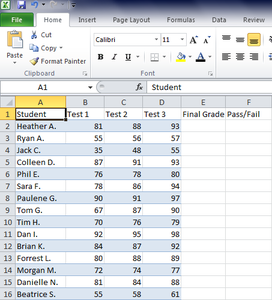
1.) In cells A1-A16, enter the following text in order starting at the top of the column, moving downward: Student, Heather A., Ryan A., Jack C., Colleen D., Phil E., Sara F., Tom G., Paulene G., Tim H., Dan I., Brian K., Forrest L., Morgan M., Danielle N., Beatrice S., and Class Average

2.) In cells B1-B16, enter the following text and numbers in order starting at the top of the column, moving downward: Test 1, 81, 55, 35, 87, 76, 78, 90, 67, 70, 92, 84, 80, 72, 81, and 55.

3.) In cells C1-C16, enter the following text and numbers in order starting at the top of the column, moving downward: Test 2, 88, 56, 48, 91, 78, 86, 91, 87, 76, 95, 87, 88, 74, 84, and 58.

4.) In cells D1-D16, enter the following text and numbers in order starting at the top of the column, moving downward: Test 3, 93, 57, 55, 93, 80, 94, 97, 90, 79, 98, 92, 89, 77, 88, and 61.

5.) In cell E1, enter Final Grade, and in cell F1, enter Pass/Fail.
   -Data for columns E and F will be entered later in the Formulas and Functions section.

*Note: Feel free to enter some of the data horizontally along the row, instead of vertically down the column, to get practice with the different keyboard functions.

Once all the data is entered, your spreadsheet should match the image above.

Step 4: Formatting

Formatting Data

There are many different options in Microsoft Excel to format numbers, text, and the cells themselves. These instructions will cover some of the more basic and widely-used formatting options available:

Changing the Font

Font commands will allow you to change the style, size, or color of the text you wish to alter:

Style

1.) Select the cells you wish to modify.
     -In this case, please select all data.

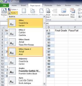
2.) To change the font style of the cells as well as the row and column headers, click on the PAGE LAYOUT tab at the top of the page

3.) Click the drop-down arrow next to the FONT command in the upper left corner of the screen

4.) Scroll over the various fonts and choose “Office Classic 2-Arial-Arial”

*Note: to change the font of ONLY the cells and not the row and column headers, complete the same directions just given, only under the HOME tab at the top of the page.

Size

1.) Select the cells you wish to modify
     -In this case, please select cells A1-F1 (Column Headers).

2.) Under the HOME tab at the top of the page, locate the drop-down arrow next to the font size command

3.) Click on the drop-down arrow

4.) Scroll over the various font sizes and choose size 12.

Color

1.) Select the cells you wish to modify
     -In this case, select cells A1-F1 again.

2.) Under the HOME tab at the top of the page, locate the drop-down arrow next to the font color command.

3.) Click on the drop-down arrow

4.) Scroll over the various font colors and click on the desired color

Step 5: Text Alignment

 Horizontal

1.) Select the cells you wish to modify
     -In this case, please select all cells.

2.) Under the HOME tab, you can one of the three horizontal alignmentcommands
      • ALIGN TEXT LEFT: aligns text to the left of the cell
      • CENTER: aligns text to the center of the cell
      • ALIGN TEXT RIGHT: aligns text to the right of the cell

Vertical

1.) Select the cells you wish to modify
     -In this case, please select all cells.

2.) Under the HOME tab, select one of the three vertical alignmentcommands
      • TOP ALIGN: Aligns text to the top of the cell
      • MIDDLE ALIGN: Aligns text to the middle of the cell
      • BOTTOM ALIGN: Aligns text to the bottom of the cell
          -In our example, we used Middle alignment for both Horizontal and Vertical.

Step 6: Numbers and Dates

1.) Select the cells you wish to modify

2.) Under the HOME tab, find the formatting section labeled NUMBERS

3.)  Click on the drop-down arrow and select the number format you want (some frequently used examples include Currency, Time, Date, Percentage, Fraction, etc.)

Step 7: Entering a Table

Returning to our previous example from the instructions regarding data entry, follow these steps to further format the data and text you entered:

1.) Use your mouse to highlight all the cells containing text or number data

2.) Click on the INSERT tab at the top of the page and select TABLE

3.) Make sure you click on the box (you will see a checkmark appear) stating that the table has headers

4.) Click on the OK button to finalize the formatting

*Note: Feel free to also format other aspects of your spreadsheet discussed above such as the style, size, and color of the font to fit your own preferences.

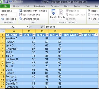
Step 8: Your Spreadsheet Should Now Look Like This:

Step 9: Formulas and Functions

Once you have a column of numbers, there are several different calculations you can do with these.

Average and Sum

1. Type in Class Average in cell A17 and change the font color to red.

2. Select the cell in which you want the average to appear. In this case, B17

3. Type =average(

4. Click and drag over the cells that you want to be averaged. In this case, B2-B16.

5. A moving border will appear around all the cells that are going to be averaged. When you have the right cells selected, hit ENTER.

6. Repeat steps 1-5 for columns C and D.

7. Change font color of B17, C17, and D17 to red to match A17.

*Note: If you want to add the total of a row or column, you can follow the same steps but instead of the word ‘average’ insert the word ‘sum’ so when you select the cell you want the sum to be in, you will type =sum(

Step 10: Rounding Numbers

Now you can go back and format the cells to make them currency or to round them to 2 decimal points.

1. Right click on the cell that has the average in it, as averages typically have many decimal points.

2. Click Format Cells...

3. On the left box, select Number

4. On the right side, make sure the box after Decimal Places: says 2

Step 11: Formulas Extending Multiple Rows/Columns

In order to extend a formula over multiple cells, first type the formula in one cell. In this case, we will put the average in column E.

1. In cell E2 type =average(

2. Click and drag to select cells B2 C2 and D2

3. Hit ENTER

4. The formula should have extended throughout all of column E to insert the average of each student and the class average.

5. Select cells E2-E17 and format the cells so that they are rounded to 2 decimal places.

Step 12: At This Point Your Table Should Match the Picture Below:

Step 13: If Formula

Now we will use Excel to help show us which students have passed and which have failed.

1. Select cell F2

2. Type =if(E2<60, “Fail”, ”Pass”)

3. Hit ENTER

4. The formula should extend throughout column F to complete which students have passed or failed.

Step 14: Conditional Formatting

Now we will use Conditional Formatting to visually highlight who has failed.

1. Click and drag on cell F2 all the way to cell F16

2. On the HOME tab, click on Conditional Formatting > Highlight Cells Rule > Text that Contains…

3. A box will pop up, type in Fail and select Light Red Fill with Dark Red Text

4. Hit OK

5. Now all the Fail grades should be highlighted in red.

Step 15: Here Is a Video to Help With Any Questions About Formulas:

Step 16: Your Spreadsheet Should Now Look Like This:

Step 17: Graphs: Scatterplot

Scatterplot Graph

1. Highlight data and titles required.
     -In this case, select columns A-E up to cell 16 in each. Student, Test 1, Test 2, Test 3, and Final Grade should be highlighted.

2. Click on INSERT on the ribbon.

3. Select Scatter from the Charts section.

4. Click scatterplot type needed

5. After the scatterplot graph shows up, click on the graph and move it to desired place on the spreadsheet.
     -In this case, the Scatterplot will be moved under the Table

Step 18: Graphs: Line Graphs

Line Graph

1. Highlight data and titles required.
     -In this case, select columns A-D up to cell 16 in each. Data from Test 1, Test 2, and Test 3 for each student should be highlighted.

2. Click on INSERT on the ribbon.

3. Select Line from the Charts section.

4. Click which line graph type is needed

5. After the line graph shows up, click on the graph and move it to desired place on the spreadsheet.
     -In this case, the line graph will be moved to the right of the scatterplot graph.

Step 19: Graphs: Bar Graphs

Bar Graph

1. Highlight data and titles required.
     -In this case, select B17-E17. The Class Averages for Test 1, Test 2, Test 3 and Final Grade should be highlighted.

2. Click on INSERT on the ribbon.

3. Select Bar from the Charts section.

4. Click which bar graph type needed

Step 20: Graphs: Titles

How to Add Titles:

1. Select a graph by clicking on it.
     -In this case, click on the scatterplot graph.

2. A “Chart Tool” bar should appear at the top center of the screen.

3. Click on the Layout tab.

4. Click on the Chart Title box.

5. Select which type of title is needed.
     -In this case, choose Above Chart

6. A text box should appear above the selected graph.

7. Fill in text box with your title
     -In this case, type in Class Grades as the title.

Step 21: Graphs: Axis Titles

Axis Titles:

1. Click on Axis Titles box
    -In this case, the bar graph will be used.
2. Select which type of title is needed.
    a. Primary Horizontal Axis Title is for the X axis
        -In this case, select Title Below Axis
    b. Primary Vertical Axis Title is for the Y axis
        -In this case, select Horizontal Title
3. A text box should appear next to the Y or X axis of the selected graph

4. Fill in text box with your title
     -In this case, the title for the X axis will be Grade, and the title for the Y axis will be Class Average.

Step 22: Switching the X and Y Axis

When using Charts or Graphs in Excel, swapping the X and Y axis can drastically change the appearance of the graphs. The following steps explain how to swap the data :

1. Select which graph you wish to alter.
    -In this case, select the bar graph.

2. Click on the Design tab.

3. In the Ribbon, click on Switch Row/Column

4. The graph design should change, and the Student Names should now be in the Y-axis, and Test 1, Test 2 and Test 3 should now be along the X-axis.

Step 23: Your Complete Spreadsheet Should Match the Following Picture: