Introduction: Streaming Sensor Data From a PpDAQC Pi-Plate Using InitialState


The Pi-PlatesppDAQC Data Acquisition and Control board is an ideal interface between sensors and a Raspberry Pi. With eight analog and eight digital inputs, up to sixteen channels of real world data can be captured by a single ppDAQC Pi-Plate. But, what can you do with that data? You can use it to control a process by turning around and driving the Digital and Analog outputs on the board. But chances are you will also want the ability to monitor it. Furthermore, the beauty of small, inexpensive single board computers (SBC) like the Raspberry Pi, is that they can be used in remote locations without a keyboard or a monitor. All they need is a source of power, and a WiFi adapter. Using a SBC in this way is referred to as a “headless” setup.
So that’s our plan: use a headless Raspberry Pi collecting sensor data in a remote location. Our options for viewing the data include:
- Watching individual readings scroll down our screen (boring)
- Saving data to a local file and then viewing the data later using a spreadsheet application or the matplotlib – sounds a lot like work
- Use InitialState to stream our data to the cloud and then look at beautiful plots of it in real time. This is how all the cool kids are doing it these days.
In this article we’re going to use option 3 to monitor two DS18B20 sensors measuring the ambient temperature in a storage closet as well as the temperature in a refrigerator used for keeping solder paste chilled.
Step 1: Stuff You Need
InitialState Access and Python Library
To begin, head to www.InitialState.com and apply for an account. While you’re waiting for approval, install their python module on your Raspberry Pi. We prefer to use pip since it makes life so easy. Go here to learn more about pip: https://pypi.python.org/pypi/pip. From the command prompt, type:
sudo pip install ISStreamer
Once you have access to the InitialState service, you’re ready to start.
Hardware
To collect the temperature data we will use the following:
- A Raspberry Pi which has been preloaded with the ppDAQC Python module. Go here if you need to perform this step.
- A ppDAQC board from Pi-Plates.com
- Two DS18B20 temperature sensors. We got ours here at Amazon.
- Two 4.7K ohm resistors. Available from Radio Shack, Digikey, and Mouser to name a few.
- Hookup wire
- A proto-board for quick and dirty or a ppPROTO for a semi permanent setup.
Step 2: Build It

Hardware
Using the materials called out in the previous step, perform the connections as shown in the drawing. Note: we were out of luck when we went looking for the 4.7K resistors so we ended up putting two 10K resistors in parallel.
Software
First you will need to create a new logging Client Key from your Initial State account. After you’ve done this, use your favorite text editor on your Raspberry Pi (this is Nano for most people) and type in the following program:
import time<br>import piplates.ppDAQC as ppDAQC
from ISStreamer.Streamer import Streamer
logger = Streamer(bucket="Lab Temperature Data", client_key="YourClientKeyHere")
logger.log("Lab Temperature Data", "Stream Starting")
while(1):
	tFridge=ppDAQC.getTEMP(0,1,'f')
	logger.log("Cooler", tFridge)
	tAmbient=ppDAQC.getTEMP(0,0,'f')
	logger.log("Ambient", tAmbient)
	time.sleep(300)
Save the above in your home directory as tempLOG.py, launch your program from the command prompt with the command sudo python tempLOG.py, and verify that no errors occur.
What’s happening in this code? Well first, we import three modules that we will need: time, piplates.ppDAQC and ISStreamer.Streamer. Then we create a stream to the InitialState data logger with:
logger = Streamer(bucket="Lab Temperature Data", client_key = "YourClientKeyHere")
After that, we go into an infinite loop and use ppDAQC.getTEMP to read the two DS18B20 temp sensors. After each read, we “log” the data along with a label to our log file at InitialState. We sleep for 300 seconds (5 minutes) and then we take another measurement.
Step 3: Examining the Log Data - Step 1
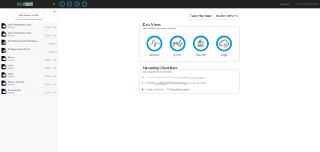
You can start looking at your data right away but there won’t be much to see until a few hours have passed. Once you’re ready, log into your Initial State account. After you’ve completed that step you’ll be taken to your own page (see image) where you can access and view your log data.
You should have a log file called “Lab Temperature Data”. Click that and then click the button that says “Source.” You will then be presented with some pretty boring lines of raw data from your Raspberry Pi that looks like:
DateTime,SignalSource,OriginalPayload
2014-12-18T15:50:57.837852Z,"Lab Temperature Data","Stream Starting"
2014-12-18T15:50:58.841351Z,Cooler,37.6
2014-12-18T15:50:59.844371Z,Ambient,69.55
2014-12-18T15:56:00.947597Z,Cooler,36.5875
2014-12-18T15:56:01.950743Z,Ambient,68.7625
2014-12-18T16:01:03.052842Z,Cooler,36.5875
2014-12-18T16:01:04.056015Z,Ambient,68.65
2014-12-18T16:06:05.104770Z,Cooler,36.925
2014-12-18T16:06:06.108063Z,Ambient,68.65
2014-12-18T16:11:07.211310Z,Cooler,37.6
2014-12-18T16:11:08.214343Z,Ambient,68.65
2014-12-18T16:16:09.319658Z,Cooler,38.1625
2014-12-18T16:16:10.322882Z,Ambient,68.65
2014-12-18T16:21:11.426134Z,Cooler,38.6125
2014-12-18T16:21:12.429228Z,Ambient,68.65
Not very interesting is it.
Step 4: Examining the Log Data - Step 2

Now click the “Wave” button and you should see something much prettier. Here is what I had after about 18 hours of monitoring. To get this plot, I went into the Tools (that little gear icon) and hid the first line labeled “Lab Temperature Data.” Then, while still in Tools, I used the Amplify Signal+ feature to increase the size of each “waveform” until they filled the screen. Then, I clicked on the “Units” button and selected hours. Finally, I dragged to cursors to the beginning and end of the log.
So now we have our pretty plot courtesy of InitialState. The refrigerator data is on the top and the closet temperature is on the bottom. What conclusions can we draw?
- The refrigerator cycles the compressor periodically to maintain the temperature. By dragging the cursors to the appropriate locations we can measure the period of this cooling cycle as 0.6 hours or 36 minutes.
- Also, by dragging the cursor we can see that the refrigerator temperature swings from about 36.5 to 38.6 degrees Fahrenheit. This is good for solder paste but not so much for beer.
- We can observe that at about the 11 hour mark, the thermostat in the lab switched to night mode and the closet temperature started to ramp down.
- We can observe that about the 18 hour mark, the heat came back on and the closet temperature started ramping back up.
- The most interesting thing though is the fact that the cooler temperature droops a little during the night. This indicates a lack of good temperature regulation and a waste of energy.
Step 5: Examining the Log Data - Step 3

There are more toys to play with on your log page. With one of your waveforms selected, click on the “Stats” button. On the left is a detailed histogram of all of the Cooler data as well as some basic statistical values. Here we can see our maximum, minimum, and average values. While the average is 37.28 degrees, the histogram also tells us the values 36.54 to 36.69 occur most frequently – this measurement is called the “mode”. The chart on the right also reflects the mode data.
Step 6: Wrap Up
In this example we learned how to connect the DS18B20 temperature sensor to a Pi-PlatesppDAQC, how to stream the data to a log file at InitialState.com, and how to manipulate and examine our data after we streamed it.
This is just a simple example of what can be accomplished with these simple components. There’s plenty of other phenomena that can be measured and logged- things like humidity, sound, light, air pressure, resistance, distance, voltage, current, weight, and strain just to name a few.