Introduction: Using an Arduino and Python to Plot/save Data


A quick and easy way to see (and then save) data taken using an Arduino onto your computer.
(Note: not the most robust method, but it works well enough)
Materials:
- Arduino (I’m using an Uno)
- Computer (I have a Dell, but it shouldn’t really matter if you are running Windows. Otherwise, you’ll need to make some minor edits to the Python code.)
- Python, including the matplotlib, pyserial, and numpy extensions
http://matplotlib.org/downloads.html (matplotlib)
https://pypi.python.org/pypi/pyserial (pyserial)
http://www.scipy.org/scipylib/download.html (numpy)
- Some sort of sensor/input device (I’m using an ADXL335 accelerometer)
- Wires/breadboard
Step 1: Wiring the Circuit
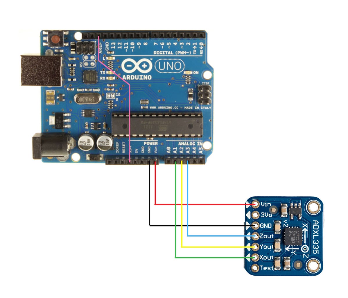
This accelerometer is extremely simple to use. It is powered off of 5VDC and each output pin (X, Y, Z) gives an analog voltage from 0-3V depending on the measured acceleration. To power it, simply connect the 5V output pin and one of the GND pins of the Arduino to the Vin pin and GND pin on the accelerometer. The X, Y, and Z pins go to any three of the analog input pins on the Arduino (I used A1, A2, and A3).
You can leave the setup like this, but the analog pins on the Arduino range from 0-5V, while the accelerometer ranges from 0-3V. This means that you will only be using about half of the range of possible analog values and will have less precision in your measurements. Ideally, the ranges would be the same so the full range of analog values is available.
The Arduino range can be changed by connecting a new reference voltage to the AREF pin and signifying in the code that the analog reference is external (see step 2). I didn't care too much about precision, so I just used the 3.3V output on the Arduino as my reference voltage, but the 3V output on the accelerometer should work as well.
Step 2: Arduino Code
The Arduino simply reads in the values on all three analog pins and sends them over serial to the computer. Tabs are added between the data to make it easier to read on the computer side.
The only setup required (other than declaring variables) is to create the serial connection at a baud rate of 9600 and declare the analog reference to be external, as mentioned earlier.
{{{
/*
This code reads in values on analog pins A1-A3 and sends the values
over serial. The outputs can be checked using the serial monitor.
created 03/18/14
*/
const int xpin = A3; // x-axis
const int ypin = A2; // y-axis
const int zpin = A1; // z-axis
void setup()
{
Serial.begin(9600); //setup serial connection
analogReference(EXTERNAL); //set external reference point for analog pins
}
void loop()
{
Serial.print(analogRead(xpin)); //read xpin and send value over serial
Serial.print("\t"); //send a "tab" over serial
Serial.print(analogRead(ypin));
Serial.print("\t");
Serial.print(analogRead(zpin));
Serial.println(); //ends the line of serial communication
delay(100);
}
}}}
Step 3: Python Code
The Python code reads the incoming serial data, and separates each line along the tabs, giving you separate values for the X, Y, and Z data. Some processing is done to put the values into their own variables.
To plot the variables, the “matplotlib” library is used to create an animated graph. This results in a reasonably accurate “live feed”, but large amounts of sensor activity will cause the graph to lag a bit.
Finally, the data is saved to a .txt file in a specified location. The data can then be read back when needed using the numpy.loadtxt() function (see next step for code). However, this file type is most easily read in Python, so if you want to open the data in a different program you’ll need to use a different write function. (ex. Use .csv file format to open data in Excel) Don't forget to change the file location to match your computer's directory.
See the code for more detailed comments (or Google or ask and I’ll do my best to explain or point you to an explanation)
{{{
'''
Reads in data over a serial connection and plots the results live. Before closing, the data is saved to a .txt file.
'''
import serial
import matplotlib.pyplot as plt
import numpy as np
import win32com.client
connected = False
#finds COM port that the Arduino is on (assumes only one Arduino is connected)
wmi = win32com.client.GetObject("winmgmts:")
for port in wmi.InstancesOf("Win32_SerialPort"):
#print port.Name #port.DeviceID, port.Name
if "Arduino" in port.Name:
comPort = port.DeviceID
print comPort, "is Arduino"
ser = serial.Serial(comPort, 9600) #sets up serial connection (make sure baud rate is correct - matches Arduino)
while not connected:
serin = ser.read()
connected = True
plt.ion() #sets plot to animation mode
length = 500 #determines length of data taking session (in data points)
x = [0]*length #create empty variable of length of test
y = [0]*length
z = [0]*length
xline, = plt.plot(x) #sets up future lines to be modified
yline, = plt.plot(y)
zline, = plt.plot(z)
plt.ylim(400,700) #sets the y axis limits
for i in range(length): #while you are taking data
data = ser.readline() #reads until it gets a carriage return. MAKE SURE THERE IS A CARRIAGE RETURN OR IT READS FOREVER
sep = data.split() #splits string into a list at the tabs
#print sep
x.append(int(sep[0])) #add new value as int to current list
y.append(int(sep[1]))
z.append(int(sep[2]))
del x[0]
del y[0]
del z[0]
xline.set_xdata(np.arange(len(x))) #sets xdata to new list length
yline.set_xdata(np.arange(len(y)))
zline.set_xdata(np.arange(len(z)))
xline.set_ydata(x) #sets ydata to new list
yline.set_ydata(y)
zline.set_ydata(z)
plt.pause(0.001) #in seconds
plt.draw() #draws new plot
rows = zip(x, y, z) #combines lists together
row_arr = np.array(rows) #creates array from list
np.savetxt("C:\\Users\\mel\\Documents\\Instructables\\test_radio2.txt", row_arr) #save data in file (load w/np.loadtxt())
ser.close() #closes serial connection (very important to do this! if you have an error partway through the code, type this into the cmd line to close the connection)
}}}
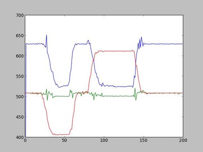
Step 4: Results
This is just the most basic plot - you can easily add axes labels, legend, etc. using matplotlib (just Google for it). I simply rotated the X axis to +/-1g for this test. When it's running, the plot will update constantly to show live movement.
Step 5: Reading Back the Data

To read back the data saved with numpy.savetxt(), you use numpy.loadtxt() and assign it to a variable. The variable can then be manipulated and re-plotted (in my case, I have the "markers" option set so I can see the individual data points).
{{{
'''
Reads and plots data from a .txt file
'''
import matplotlib.pyplot as plt
import numpy as np
#load values from file into "data"
data = np.loadtxt("C:\\Users\\me\\Documents\\Instructables\\test.txt")
#create empty lists for data to be sorted into
x = []
y = []
z = []
#for each line in data, sort it into the appropriate list
for dat in data:
x.append(dat[0])
y.append(dat[1])
z.append(dat[2])
#plot each list then show the plot
plt.plot(x, marker = 'o')
plt.plot(y, marker = 'o')
plt.plot(z, marker = 'o')
plt.show()
}}}

Participated in the
Data Visualization Contest