Introduction: Pier 9 Guide: Beginner and Advanced CAM Programming


This Instructable is for Workshop Users at Pier 9. It was originally written by Dan Vidakovich.
This Instructable is a detailed, step-by-step set of instructions to show you how to program a part using CAM (Computer Aided Manufacturing). Using Autodesk's Inventor Pro HSM 2016, you will learn how to prepare a part for machining in aluminum on a 3-axis CNC machine--at Pier 9, the Haas CNC VF2SS Mill!
This certification part will introduce you to facing, contour, adaptive, and pocket toolpaths. You'll learn how to drill holes using custom tools, prepare multiple setups, and prepare for flip machining. By practicing this process, you'll have the skill set to prepare many of your own custom designs for CNC machining.
Ready to make chips fly?
Step 1: Beginner CAM Programming - Introduction to Autodesk Inventor HSM Pro 2016

CAM software creates instructions for the machine to make your part, called toolpaths. We'll be creating toolpaths using Autodesk Inventor HSM Pro 2016.
Visit cam.autodesk.com and download and install a trial version of Autodesk Inventor HSM Pro 2016.
Step 2: Setup - Work Coordinate System (WCS)


There are three steps in the CAM process: Setup, Toolpath, & Simulate.
Setup defines the Work Coordinate System (WCS) and the size of your raw material (stock).
Setup
1. Open the attached file 'Haas_certification_part_your_name_here.ipt'
2. In the tabs at the top, click the CAM tab. This tab contains controls for fully integrated CAM.
Note: Autodesk Inventor HSM buttons are positioned like reading a book: you'll most likely use buttons starting from the left and moving to the right.
3. On the ribbon, click Setup.
Work Coordinate System (WCS)
Peter Smid defines WCS in his CNC Programming Handout on page 127:
"Work offset is a method that allows the CNC programmer to program a part away from the CNC machine, without knowing its exact position on the machine table."
In the graphics window, the box surrounding the model contains many points or nodes. These points are potential locations for the WCS. The default position for the WCS is in the center of the part.
4. In the graphics window, click the upper left point/node. This moves the WCS to the upper left corner and defines the X, Y, and Z coordinates of the WCS.
Note: The x-axis points along the long axis of the part, the y-axis points away, and the z-axis points up.
This X, Y, and Z orientation is important and we'll need to remember this when we place our stock in the CNC machine. For a more detailed explanation of the Work Coordinate System, watch this video Setting up a Work Coordinate System and read Chapter 4, Coordinate Systems, in the CNC Handbook.

Step 3: Setup - Stock


Setup
1. With the Setup dialogue still open, click the Stock tab.
Note: By default, stock material evenly surrounds the part. The stock dimensions are: 6" x 4" x 1.5". Raw material is usually thicker, so our z-dimension is 2 inches rather than 1.5 inches.
2. In the Height (Z) field, change 1.5 to 2.
3. In the Model Position drop down menu, click Offset from Top (+Z). This allows you to position the model inside the stock.
4. In the Offset field enter 0.05. This offsets our model 0.05 inches below the top of the stock.
Note: Our stock dimensions are now 6" x 4" x 2".
5. Click OK to close the Setup dialogue box.
Note: On the left side of the screen, notice Setup1 in the CAM Feature Tree. The CAM Feature Tree contains Setups and Toolpaths organized in a hierarchical order. Setup is the highest (or parent) level and toolpaths are dependent (children). To edit an existing Setup, right-click and choose edit or simply double-click.
Step 4: Install Pier 9 CNC Tool Library

1. Download two files: 'Adaptive Clearing Formula Nov16' and the latest Haas Mill Tool Library, labeled on
the sticker outside the machine and available for download from the Pier 9 CNC Data Instructable.
The naming convention is: P9_haasMill_lib_MonthYear.hsmlib
2. In Windows explorer, create a new folder on your hard drive called 'Pier 9 CNC Tool Libraries' and save both files. We'll use the Adaptive Clearing Formula to do something really cool later on.
3. On the right side of the CAM ribbon, click Tool Library. This opens the tool library dialogue.
4. Click My Libraries folder.
5. In the bottom left corner, click New Library and name this library 'P9_HaasMill_monthYear.hsmlib'. This creates a new, and empty, tool library which we will use to import tools.
6. Right-click this newly created library and click ImportTools from Library.
7. Browse to the tool library you just saved on your hard drive and click Open.
8. Click OK to close the Tool Librarydialogue.
Note: Any changes made in the Tool Library dialogue must be save by clicking OK.
You just installed the Pier 9 Haas CNC Mill library! You'll find it very useful for programming your parts at the convenience of your desk.
Step 5: Facing Toolpath

Next, let's create a Toolpath.
Face milling from the CNC Programming Handbook on page 235:
"Face milling is a machining operation that controls the height of the machined part. For most applications, face milling is a relatively simple operation, at least in the sense that it usually does not include any special contouring motions. Cutting tool used for face milling is typically a multi tooth cutter, called a face mill, although end mills may also be used for certain face milling operations, usually within small areas. Top surfaces machined with a face mill are generally perpendicular to the facing cutter axis."
1. On the Ribbon in the 2D Milling section, click Face.
2. Click Tool
3. In the My Libraries section, click P9_HaasMill_monthYear tool library.
4. Select Tool 171 2" Face Mill
5. In the bottom right, click Select. This closes the Tool dialogue.
6. Click OK at the bottom of the Face dialogue. This creates your first toolpath, facing. The lines in the graphics window are called toolpaths.
Note: Face toolpath is extremely simple because it removes all material from model top to stock top.
7. Read about Facing the CNC Handbook.
Concept Check:
How much stock material was removed during facing? If you don't know the answer, take a closer look at the Setup step.
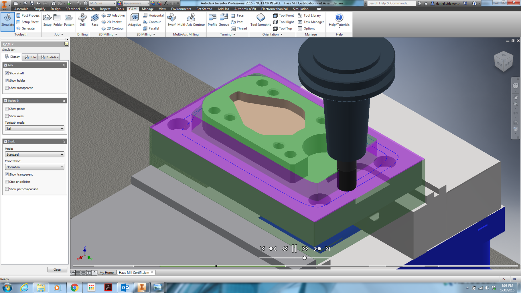
Step 6: Simulate

Simulate
Next, Simulate the facing toolpath.
1. On the Ribbon, Click Simulate.
2. In Toolpath mode, click Tail.
3. Put a check mark in the Stock box.
4. Put a check mark in Show transparent.
5. Click Play in the bottom middle of the screen.
Note: Simulation is extremely important and is exactly what the machine will do. Pay close attention to details such as: What side of the part does the tool start? What is the thickness of material removed?
Ensure you understand each machine movement and why. During programming, you'll spend 50% of your time in simulation to ensure proper tool placement and toolpath settings.
6. Click Close.
Step 7: The CAM Mantra

Setup, Toolpath, Simulate - That's the workflow for programming CNC machines. Say that four times:
Setup, Toolpath, Simulate
Setup, Toolpath, Simulate
Setup, Toolpath, Simulate
Setup, Toolpath, Simulate
Learn that and you can make anything!
Step 8: 2D Adaptive Clearing & the Formula


Next we'll remove material from the feature in the center of the part. This feature is called a pocket. The definition of a pocket by Peter Smid:
"In many applications for a CNC machining center, the material has to be removed from the inside of a certain area, bounded by a contour and a flat bottom. This process is generally know as pocketing."
There are two key words in this definition: contour and flat bottom.
1. On the Ribbon 2D Milling section, click 2D Adaptive Clearing. Adaptive Clearing creates toolpaths that removes material very quickly.
Note: On the left side of the screen, a window with five tabs opens. This is called the Toolpath Window. We'll navigate these five tabs when we first started the software - it's like reading a book, use features from the left to the right.
2. Click Tool.
3. In My Libraries section, click P9_HaasMill_monthYear. This allows us to select tools from the Pier 9 Tool Library.
4. Click #114 1/4" EM (End Mill) Short.
5. Click Geometry (the next tab to the right). This tab defines the geometry of our pocket.
Note: Recalling the definition of a pocket: "material has to be removed from the inside of a certain area, bounded by a contour and a flat bottom." By definition, we must select a contour and flat bottom. We can do this with one click thanks to the great people at HSM.
6. In the graphics window, select the bottom curve of the pocket. Clicking the bottom face of the pocket is ok, but it is more precise to select a curve.
Note: This selects the contour and flat bottom of a pocket in one click!! We did not select the upper contour of the pocket because that defines contour of the pocket but not the depth.
7. Click the Passes tab.
8. Hover your mouse over the Optimal Load field, right-click, and select Edit Expression.
9. Delete the default expression of 0.4 * tool_diameter.
10. Open the Adaptive Clearing Formula file in Notepad that you downloaded earlier (also attached at the bottom of this step) and copy/paste that formula into the Expression dialogue.
11. Click OK to close the Expression dialogue.
12. Right-click the Optimal Load field again and select Make Default. This saves the formula.
13. In the field for Maximum Roughing Stepdown, right click, and select Edit Expression.
14. Delete the default expression, and replace with the typed text: tool_fluteLength
Note: Adaptive Clearing is unique and efficient because you can use the entire length of the flutes in a single stepdown. This formula saves you the labor of editing the tool to check the flute length, and then entering that number in this field.
15. Right-click the Maximum Roughing Stepdown field again and select Make Default. This saves the formula.
16. Click OK. This generates the toolpath.
Attachments
Step 9: Adaptive Clearing Formula

The formula from the previous step was created using data from new users machining at the Autodesk Workshop at Pier 9.
In the image above, the graph on the top left plots the default value of tool diameter vs. optimal load. This line was generated using the default formula of 0.4 * tool_diameter that ships with the software. It's slightly over-simplified and does not take into account the maximum power of your CNC machine. As tool diameter increase above 5/8", so does the power required to cut with the entire length of the cutting flutes. From experience, 5/8" diameter tools using the default formula and cutting aluminum use the maximum power available of our Haas VF2 SS mill (30 horsepower).
The graph on the top right displays the metal removal rate if we reduce optimal load for tools larger than 5/8". The removal rate goes down, but it's much safer and we haven't had any parts come out of the vise or broken 1" diameter tools (which are also very expensive).
In the graph on the bottom, the blue line represents adjusted values of optimal load which account for machine power limitations. The orange line represents the function which fits the data. Using JavaScipt syntax, here's our new formula which makes things be a little more automated and safer:
(Math.min(-1.046*tool_diameter/(25.4*25.4)*tool_diameter*tool_diameter + 0.874*tool_diameter*tool_diameter/25.4 + 0.209*tool_diameter + 0.01in;0.5 * tool_diameter))/(1.5)
Step 10: Simulate 2D Adaptive Clearing


1. In the CAM feature tree, click Setup1. This simulates all toolpaths in the Setup.
2. On the Ribbon, Click Simulate.
Note: Tail mode, Stock, and Show Transparent are already checked.
3. Click Play.
4. Click >0. This skips to the next toolpath, 2D Adaptive.
Remember: Setup, Tool Path, Simulate. It's that easy!
5. Click Close. This closes the simulation.
6. Click Save to save the toolpaths.
Step 11: 2D Pocket (Finishing)


Now that we've quickly roughed out our part, let's program a finishing pass.
1. On the Ribbon 2D Milling section, click 2D Pocket.
Note: The tool from the previous operation, #114 1/4" EM Short, is selected by default.
2. In the graphics window, click the bottom curve of the pocket. This defines the pocket boundary (contour) and depth (flat bottom).
Note: By default the software is prepared for a geometry selection, so there's no need to click the Geometry Tab.
3. Click the Passes Tab.
4. Uncheck Stock to Leave since this is a finishing tool path.
5. Click OK.
6. Inspect your tool paths. This is a finishing tool path which machines the bottom and sides to the final dimension.
7. In the CAM Feature Tree, click Setup1.
8. On the Ribbon, click Simulate.
9. Click Play.
10. Adjust the slider below the play button to speed up the simulation.
Note: Each toolpath is assigned a unique color during simulation.
11. Click Close to close the simulation.
12. Read about pocketing in the CNC Handbook.
Step 12: 2D Adaptive Clearing


The next 2.5D milling operation quickly removes material from the outer portion of the part.
1. On the Ribbon, click 2D Adaptive Clearing.
2. Click Tool.
3. In My Libraries, click P9_HaasMill_monthYear tool library.
4. In the tools window, click #132 1/2" Rough End Mill (EM) Short.
5. Click Select.
6. In the graphics window, hover your mouse over the outer contour of the raised feature in the center until the geometry turns light blue.
7. Click the light blue contour. The geometry now turns dark blue and a shaded box appears.
Note: It is important to take your time and be precise when selecting geometry. In this case, precision is necessary to select the contour and not the lower face. Selecting the lower face does not machine all stock material.
8. In the graphics window, click the contour of the small open pocket on the right side. This selects the open pocket at a slightly deeper depth.
Note: An open pocket is a pocket which is partially surrounded by material.
9. Click the Passes tab. Notice Stock to Leave is enabled by default because this is our roughing toolpath.
10. Click OK. This generates the 2D Adaptive Clearing toolpath.
11. On the CAM Feature Tree, click Setup1. This selects all toolpaths.
12. On the Ribbon, click Simulate.
13. In the middle of the screen, click Play.
Note: It is not visible in Simulation, but coolant is enabled by default. All Pier 9 CNC Tool Library tools have flood coolant enabled by default. It is important to enable flood coolant during Adaptive Clearing because Adaptive Clearing generates heat and chips and these must be removed with flood coolant.
14. To advance toolpaths, near the bottom of the screen click on the super-thin, hard-to-find little gray bar, called the Timeline. This jumps to a spot in the simulation.
Note: Hover your mouse over the timeline for helpful statistics.
15. Click Close to close the simulation.
Step 13: Adaptive Clearing Definition

Adaptive Clearing is a High Speed Machining (HSM) toolpath which maintains a constant load or force on the cutting tool. This constant and predictable load on the cutting tool enables CNC programmers to utilize the entire cutting flute which results in high metal removal rates, reduced cycle time, and reduced tool wear. Flood coolant is recommended during Adaptive Clearing High Speed Machining.
Step 14: 2D Pocket (Finishing)


Adaptive Clearing quickly removed most material. Perform a finishing pass to machine the part to the final dimension and leave a smooth finish.
1. On the Ribbon, click 2D Pocket.
2. In the graphics window, click the same outer contour of the raised feature in the center and the small open pocket on the right side.
Note: We did not select a new tool. By default, Inventor HSM uses the same tool, #132 1/2" EM Short, from the previous operation.
3. In the toolpath dialogue, click the Passes tab.
4. Uncheck stock to leave.
5. Click OK. This generates a finishing toolpath.
6. On the Ribbon, click Simulate.
Note: We intentionally did not click Setup1 prior to clicking Simulate. Doing this simulates the last toolpath created and is not a recommended practice.
7. In the middle of the screen, click Play. Notice the 2D pocket toolpath simulation is the only one displayed. In this case, this is simulation is not helpful.
8. Click Close to close the simulation.
9. In the CAM Feature Tree, click Setup1.
10. Click Simulate.
11. Click Play.
Note: This displays all the operations in Setup1 and is a recommended practice.
12. Click Close.
13. Click Save to save the toolpaths.
Step 15: 2D Pocket Definition


2D Pocket is a toolpath which uses the selected geometry, not optimal load, to create concentric toolpaths. This results in variable and unpredictable peak loads on the cutting tool which must be mitigated by cutting at multiple depths.
Unlike 2D Adaptive Clearing, 2D Pocket does not generate constant loads or forces on the tool. This variable load is low enough for light finishing passes, but is not suitable for high speed roughing passes. As a result, use 2D Pocket for light finishing passes and 2D Adaptive Clearing for High Speed Machining (HSM).
Step 16: Spot Drill Rule


Prior to drilling a hole in metal, first use a spot drill (or center drill) to make a starter hole. The depth of the starter hole = Hole Diameter/2. (or Starter Hole Depth is equal to the radius of the final hole to be machined)
Begin by spot drilling the four counterbored holes on the perimeter. The counterbore is the larger hole, closer to the surface of the part, and the bore is the smaller hole, deeper in the part.
1. In the upper level row of tabs at the top, click Inspect.
2. On the Ribbon, click Distance.
3. In the graphics window, click on the body of the outer hole below the counterbore. The diameter is 0.354".
Note: Zoom in and rotate the model as necessary to accurately select the hole diameter. One option is to click Tool Top to clearly measure the diameter of the hole (these are the only holes that go all the way through the model).
4. In the distance window, click the arrow.
5. In the drop down menu, click dual unit.
6. Click millimeters.
The diameter of this hole is 0.354" or 9 mm. The depth of the starter hole will be 0.177" or 4.5mm.
7. Read about spot drilling (center drilling) in the CNC Handbook.
Step 17: Spot Drill


1. Return to the integrated CAM environment. Click the CAM tab.
2. Click Drill.
3. Click Tool.
4. In My Libraries, clickP9_haasMill_monthYear.
5. Click tool #131 1/2" Drill Mill
6. Click Select.
7. In the graphics window, select the counterbore.
Note: Look closely at the image above to ensure you selected the correct geometry. Select the larger hole (the counterbore) and not the smaller hole (the bore or hole).
8. In the Drill Toolpath Window, check Select same diameter.
9. In tabs, click the Heights tab.
10. In the Bottom Height section, click the drop down and select Hole top.
11. In the Bottom Offset, input -0.177 in (Depth of starter hole calculated in the previous step).
12.Click OK to generate the toolpath.
13. In the CAM Feature Tree, click Setup1.
14. On the Ribbon, Click Simulate.
15. Instead of clicking Play, click >|. This jumps to the end of the simulation and displays the machined part.
Note: Proceeding to the end of the simulation is processor intensive. If there are many toolpaths this may take a few moments. Please be patient. For faster rendering, in the Simulation Window Stock section, click the Mode drop down and select Fast (3-axis only).
16. Click Close to close the simulation.
Note: It is important to always close CAM dialogue windows before using CAD tools such as 3D Model or saving the model. If the software crashes, please submit a crash report.
Step 18: Spot Drill Remaining Holes


To spot drill the eight remaining holes, there's a handy trick using the countersink or chamfer at the top of the hole.
1. On the Ribbon, click Drill.
Note: We did not select a new tool. By default, Inventor HSM uses the same tool, #131 1/2" Drill Mill, from the previous operation.
2. In the graphics window, click the angled surface (countersink) for two the different diameter holes in the center of the part. Please reference the picture above.
Note: There's no need to click the Geometry tab, because the software anticipates a geometry selection by default. This speeds up the programming process.
3. Check Select same diameter. This selects the eight holes on the top of the part.
4. Click OK to generate the toolpath.
5. In the CAM Feature Tree, click Setup1.
6. On the Ribbon, click Simulate.
7. Click Play.
8. In the Simulation Window, click the Info tab. Notice the feeds & speeds, machine time for the current operation, and collision detection information.
9. Click Close to close the simulation.
Step 19: Drill Outer Holes


The four outer holes with counter bores are 9mm in diameter and 20mm deep.
Calculate the depth to diameter ratio: 20/9 = 2.222.
1. On the Ribbon, click Drill.
2. Click Tool.
3. In the Sample Libraries section, click ISO Drills.
4. Click on the 9mm drill.
5. Click Select.
6. Click Tool again. In the Open Documents section, notice the 9mm sample library drill was automatically assigned a tool number.
7. Right-click the 9mm drill and select Edit.
8. In the General tab (Post Processor tab in Fusion) change the Tool Number to 1.
Note: The drill may already be assigned a tool number. The number automatically assigned depends on the order in which it was picked.
Note: Length Offset and Diameter Offset should also be assigned a 1 automatically. It's important that these match so don't change them, or there could be some serious machine damage. Don't make this mistake.
9. Click the Coolant dropdown and change it to Flood.
11. In the Description field type "9 mm Drill". This will help you identify the tool later.
12. Click the Feed & Speed tab.
Change the Surface Speed to 80 ft/min to input the correct RPM.
Don't forget to include units. You can also use 25 m/min.
13. Enable Flood Coolant.
14. Change the Feed per Revolution to 0.002 in.
Don't forget to include units. You can also use 0.050 mm.
15. Click OK. Click Yes in the popup and OK in the second popup.
16. Click Select to select the 9mm drill with the new tool number and speeds and feeds.
Note: In the Tool tab, notice the new tool data is displayed.
17. In the graphics window, select one of the 9mm holes on the perimeter.
18. Check Select same diameter. This quickly selects the remaining three holes.
19. Click the Heights tab.
20. In the Top Height section, click the drop down and choose Selection.
21. In the graphics window, click on the surface at the top of the counter bore. This sets the drill start height.
22. In the Bottom Height section, check Drill tip through bottom box. Change Break-through depth to 0.05 in. This ensures the drill tip drills deeper than the hole bottom making the full diameter of the hole.
23. Click the Cycle tab.
24. Hover your mouse over the Cycle type down menu. A popup with helpful drilling information and cycle types appears.
Note: The depth to diameter ratio for this hole is 2.222, therefore, we will use the default cycle, Drilling - rapid out. If the depth to diameter ratio is greater than three, the hole must be drilled using a special drilling cycle called deep drilling - full retract (or peck drilling). This prevents the drill from breaking by drilling only a fraction of the hole depth at a time and fully retracting the drill to remove chips. Since the depth to diameter ratio for this hole is less than three, the standard drilling cycle, Drilling - rapid out, is used.
25. Click OK to generate the toolpath.
26. On the Ribbon, in the Orientation section click Tool Front.
27. Zoom in and visually inspect the tool path. The green drilling toolpath should extend below the part.
28. On the Ribbon, click Simulate.
29. Click Play. Watch the simulation.
Note: Even though this toolpath extends beyond our part, it does NOT cut through our stock. Initially, we chose stock material that was much thicker than our part.
30. Click Close to close the simulation.
31. Read about Drilling in the CNC Handbook.
32. Click Save to save the toolpaths.
Step 20: Drill Middle Holes


The next set of holes are 8 mm in diameter and 20 mm deep.
The depth to diameter ratio is 20/8 = 2.5
1. On the Ribbon in the Orientation section, click Tool Isometric. This orients the part in an isometric view based on your Work Coordinate System (WCS).
2. On the Ribbon, click Drill.
3. Click Tool.
4. In the Sample Libraries section, click ISO Drills.
5. Click 8 mm drill.
6. Click Select.
7. Similar to the previous step, Click Tool again.
8. In the Open Documents section, Right-click the 8mm drill and select Edit.
9. In the General tab (Post Processor tab) change the Tool Number to 2.
10. Click the Coolant dropdown and change it to Flood.
11. In the Description field type "8 mm Drill".
12. Click the Feed & Speed tab. Change the Surface Speed to 80 ft/min to input the correct RPM.
Don't forget to include units. You can also use 25 m/min.
13. Change the Feed per Revolution to 0.002 in.
Don't forget to include units. You can also use 0.050 mm.
13. Click OK. Click Yes in the popup and OK in the second popup.
14. Click Select to select the 8mm drill with the new tool number and speeds and feeds.
15. In the graphics window, click on the body of the hole.
16. Check Selectsame diameter.
17. Click the Heights tab.
18. In the Bottom Height section, put a check mark in Drill tip through bottom. This is a little tricky: the part was 3D modeled with a conical drill tip at the bottom. We selected the hole by clicking on the hole body and not the conical drill tip. If we didn't enable Drill tip through bottom the tip of the drill would stop at the bottom of the hole body and not the tip of the conic. Investigate this for yourself by switching the model to wireframe and checking/unchecking Drill tip through bottom.
19. Click OK to generate the toolpath.
20. On the CAM Feature Tree, click Setup1.
21. On the Ribbon, click Simulate.
22. Click Play.
23. In the Simulation Window, click the Statistics tab and look at the helpful machining data.
24. Click Close to close the simulation.
Step 21: Drill Inner Holes - Deep Drilling


The next holes are 6.8 mm in diameter and 22.25 mm deep.
The depth to diameter ratio is 22.25/6.8 = 3.27. Note this ratio is greater than three.
1. On the Ribbon, click Drill.
2. Click Tool.
3. In the Sample Libraries section, click ISO Drills.
4. Click 6.5 mm drill.
Note: 6.5 mm drills are more common than 6.8 mm drills. Holes can always be enlarged after purchasing the correct drill.
5. Click Select.
6. Click Tool again.
7. In the Open Documents section, Right-click the 6.5 mm drill and select Edit.
8. In the General tab (Post Processor tab) change the Tool Number to 3.
9. Click the Coolant dropdown and change it to Flood.
10. In the Description field type "6.5 mm Drill".
11. Click the Feed & Speed tab. Change the Surface Speed to 80 ft/min to input the correct RPM.
Don't forget to include units. You can also use 25 m/min.
12. Change the Feed per Revolution to 0.002 in.
Don't forget to include units. You can also use 0.050 mm.
13. Click OK. Click Yes in the popup and OK in the second popup.
14. Click Select to select the 6.5 mm drill with the new tool number and speeds and feeds.
15. In the graphics window, click on the body of the hole.
16. Check Select same diameter.
17. Click the Heights tab
18. In the Bottom Height section, check the box Drill tip through bottom.
19. Click the Cycle tab.
20. In the Cycle type drop down, click Deep drilling - full retract.
Note: Since the depth to diameter ratio is greater than three, we must use Deep drilling - full retract - drilling cycle. For holes with depth to diameter ratios greater than three, it is difficult to completely remove chips with the standard drilling cycle, therefore, deep drilling (or chip breaking) is necessary to remove chips, prevent chips from being welded to the drill and prevent it from breaking.
21. Click OK to generate the toolpath.
22. In the CAM Feature Tree, click Setup1.
23. On the Ribbon, click Simulate.
24. Click Play.
25. Do not close the simulation. The next step will take a closer look at the completed machining operations to determine what features to machine next.
Step 22: What's Next?


With Simulation open from the previous step, let's take a closer look at the toolpaths created up to this point.
Inspect the model in the first image above. Which features are completed and which ones need to be machined? The software can help you answer this question.
1. In the Simulation window in the Stock section, check Show part comparison.
2. Inspect the model. Red indicates a gouge and blue indicates remaining stock. Pretty cool, right!?
3. Using part comparison, can you find three features that need to be machined? Can you also explain why each one exists?
Based on our part comparison analysis, we'll machine the bores next.
4. Click Close to close the simulation.
Step 23: Bore


1. On the Ribbon in the 2D Milling section, click Bore.
2. Click Tool.
3. In the Open Documents section, click Haas CNC Mill Certification. This displays the list of tools used in the current part.
4. Click #132 1/2" R0.02" bullnose Rough EM Short.
5. Click Select.
6. In the graphics window, select the four counter bores.
7. Click OK to generate the toolpath.
8. In the CAM Feature Tree, click Setup1.
9. On the Ribbon, click Simulate.
10. Click Play.
Note: Part comparison is still enabled. This assists us in identifying which features need to be machined.
Question: Why did we drill the holes before boring?
11. Uncheck Part comparison.
12. Click Close to close the simulation.
13. Click Save to save the toolpaths.
Answer: If you can, it's always a good idea to remove material with a drill. End mills don't like to plunge and removing material with a drill is easy and minimizes load on the end mill.
Another Question: If the bore diameter is slightly larger than the end mill what type of toolpath would be generated?
Step 24: Part Perimeter - 2D Adaptive Clearing


1. On the Ribbon, click 2D Adaptive Clearing.
2. Click Tool.
3. In My Libraries section, clickP9_haasMill_monthYear.
4. Click #164 1" EM Short.
5. Click Select.
6. In the graphics window, click the lower outer contour.
7. Click OK to generate the toolpath.
8. In the CAM Feature Tree, click Setup1.
9. On the Ribbon, click Simulate.
10. In the Simulate window Tool section, uncheck Show holder. This removes the tool holder from view.
11. On the Ribbon, click Tool Top.
12. Click Play.
13. Referencing the final picture above, notice the small amount of material around the perimeter of the part the simulation "thinks" it is removing. In practice this is not actually the case. While cutting our stock from a larger piece of aluminum, it is difficult to cut it exactly to size. In addition to measuring inaccuracies, sometimes the band saw cuts on an angle! We must take this into account to proceed safely.
14. Click Close to close the simulation.
Step 25: Change Setup1 - Actual Stock Size & Regenerate Toolpaths


1. Since you probably haven't actually cut any stock yet, let's take this into account and make a mental note to verify this prior to program execution.
2. Assuming minor stock cutting inaccuracies, assume our stock is 6.1" x 4" x 2". This is slightly larger than initially defined. We'll verify this after cutting stock on the band saw and before program execution.
3. In the CAM Feature Tree, right-click Setup1 and click Edit. This allows us to edit our existing Work Coordinate System (WCS) or stock size.
4. On the Ribbon, click Tool Isometric. This puts the model in a more familiar view.
5. In the Setup Window, click the Stock tab.
6. In the Stock tab, change Width (X) to 6.1.
Note: In the graphics window, the stock automatically re-sizes due to these dimension changes.
7. Click OK to accept the stock size changes.
8. In the CAM Feature Tree, notice the red x marks on each toolpath. Any changes in the Setup invalidates the toolpaths and the they must be regenerated (or recalculated) to account for this change.
Note: Reviewing the hierarchy in the CAM Feature Tree, Setup and toolpaths have a parent-child relationship. Setup is the parent and toolpaths are the children. Modifications to the parent results in changes to the child, therefore, toolpaths must be regenerated.
9. Right-click Setup1 and click Generate Toolpath (All). This regenerates (or recalculates) all toolpaths based on the new Setup stock size.
10. Click Save to save the toolpaths.
Step 26: Part Perimeter 2D Adaptive Clearing With Actual Stock Size


1. Right-click the last operation, 2D Adaptive3, and click Edit. This allows us to edit an existing toolpath.
2. Click the Passes tab.
3. Verify Optimal load is less than 0.05 in. This ensures you properly input and saved the formula from Step 8.
Note: Optimal load is the maximum load (or force) created by the 2D Adaptive Clearing toolpath. This parameter is the maximum force the tool will encounter. I know a value around 0.05 in seems low, but for large 1 inch end mills our Haas VF2 mill does not have enough horsepower. We've broken plenty of 1 inch end mills with values larger than 0.05 inches and those tools are expensive ($400!).
If the formula did not save properly, please revisit Step 8.
In the future, we won't verify Optimal load is correct each time we use Adaptive Clearing toolpaths. We did this because we needed to check if the formula was properly saved and working.
4. Click the Heights tab.
5. In the Bottom Height section, change Bottom offset to -0.05 in.
Note: Machining a little deeper than Model Bottom ensures a nice finish on the side after the part is flipped and the bottom is machined off.
6. Click OK to generate the toolpath.
7. In the graphics window, notice the extra cutting passes on either end of our part. These extra passes are the safest way to machine irregular stock. Remember, once we cut our stock material on the band saw we must measure it and update Setup1 X, Y, & Z dimensions accordingly.
8. In the CAM Feature Tree, click Setup1.
9. On the Ribbon, click Simulate.
10. Click Play.
Note: Only the tool should be visible and not the tool holder since we removed it from view in the previous step. Viewing the simulation in this way can be helpful.
11. On the Ribbon, click Tool Front.
12. Zoom in on the model. Can you explain why the Bottom offset was changed to -0.05 in?
Note: Making this part requires flipping the part and machining off the bottom. Machining -0.05 in below the bottom ensures a nice finish on the contour after the part flip.
13. On the Ribbon, click Tool Isometric.
14. Click Close to close the simulation.
Concept Check: Why machine -0.05 in deeper than Model Bottom?
Step 27: Part Perimeter 2D Contour (Finishing)


1. On the Ribbon, click 2D Contour.
Note: Our previous tool, #164 1" EM Short, was selected by default.
2. In the graphics window, click the lower and outer contour of the part.
3. In the Heights tab in the Bottom Height section, change Bottom offset to -0.05 in.
4. In the Passes tab, uncheck Stock to leave. This ensures our toolpath is a finishing toolpath and will machine our part to the final dimension.
5. Click OK to generate the toolpath.
6. In the CAM Feature Tree, click Setup1.
7. On the Ribbon, click Simulate.
8. In the Simulation window in the Stock section, check Show part comparison.
9. Click >|. This jumps to the end of the simulation and it takes a few moments to do so. In the timeline at the bottom of the screen, notice the blue progress bar which indicates the progress of generating this simulation/image.
Note: A small amount of material remains in the open pocket on the right. This is called REmaining STock, or REST, for short and we'll machine that in the next step.
11. On the Ribbon, click Tool Front.
12. Zoom in to the side of the part to visually verify the toolpath extends below the part.
Note: Visually inspecting toolpaths is a recommended practice. When machining its best to follow the guidance "Assume nothing and verify everything." Visually verifying the toolpath will give you confidence you programmed it correctly.
13. On the Ribbon, click Tool Isometric to return the part to the isometric view.
14. Click Close to close the simulation.
15. Click Save to save the part.
16. Read Chapter 7 2D Contour in the CNC Handbook.
Step 28: REST Machining


During part comparison in the previous step, it is apparent a radius was not machined. Machining this remaining material is called REST (REmaining STock) machining.
1. On the Ribbon, click 2D Pocket.
2. Click Tool.
3. In the My Libraries section, click P9_haasMill_monthYear tool library.
4. Click #103 1/8" Rough EM Long.
5. Click Select.
6. In the graphics window, click the contour of the open pocket.
7. In the 2D pocket toolpath window, check Rest Machining.
8. In the Rest Machining Section, change Tool diameter to 0.5 in. This is the tool diameter of the tool last used to machine the open pocket (#132 1/2" Rough EM Short).
Note: This parameter is confusing. Tool Diameter is the diameter of the previous tool used to machine the open pocket. This value, combined with the tool selected for this operation, 1/8" Rough EM Short, allows the software to calculate the difference between the unmanchined open pocket and the partially machined open pocket using the previous tool (i.e. subtract what was cut using previous tool from uncut open pocket). With this information, the software creates a toolpath to machine the remaining material.
That's a mouthful. If they called it "Previous Tool Diameter" instead of a non-descriptive "Tool Diameter" I would have to talk less.
9. In the Heights tab Top Height section, change the drop down to Selection and click the face above the open pocket. This changes the start height from the default Stock Top to just above to the top of the pocket.
10. In the Passes tab, uncheck Stock to Leave.
11. In the Passes tab, check Multiple Depths.
Note: Accept default values in the Multiple Depths dialogue box. At this point in your CAM training, I want you to trust CAM defaults. If you are unsure of what a setting does don't randomly change it.
10. Click OK to generate the toolpath.
11. In the CAM Feature Tree, click Setup1.
12. On the Ribbon, click Simulate.
Note: With Part comparison still checked, this might increase simulation calculation time. Please be patient.
13. Click >| and inspect the model. The top side of our model is completely machined and we are ready to flip the part and machine off the workholding (remaining) material.
14. On the Ribbon, click Tool Front and let's discuss workholding in the next step.
Step 29: REST Machining Error - Empty Toolpath


Up to this point, we've programmed the part perfectly. However, we all make mistakes and inadvertently do things that won't work...
Let's intentionally make a mistake and learn how the software handles this.
1. In Setup1, double-click 2D Pocket3, the last toolpath you created. This allows us to edit parameters of an existing toolpath. It is also acceptable to right-click the toolpath and select edit.
2. Click the Geometry tab.
3. In the Rest Machining box, change Tool diameter from 0.5 in to 0.125 in. This incorrectly changes the previous tool diameter from 0.5 in to 0.125 in.
4. Click OK to generate the toolpath.
5. In the graphics window, notice a toolpath was not generated. Incorrectly changing REST Tool diameter from 0.5 to 0.125 created a scenario in which the software cannot calculate a toolpath. This is called an empty toolpath.
6. In the CAM Feature Tree, notice the orange check mark next to 2DPocket3. This indicates a toolpath error and may result in no toolpaths generated.
7. Right-click 2D Pocket3. Select Show Log. This displays fairly cryptic messages which attempt to communicate the problem. In this case, there are two messages:
Warning: No passes to link.
Warning: Empty toolpath.
An experienced Autodesk Inventor HSM Pro 2016 software user can quickly identify and fix this error. But, I want you to show them how quickly you learn and beat them in record time by picking up all the tips and tricks in this focused Instructable.
Explaining the errors
Warning: No Passes to link. Linking connects (or links) rapid tool repositioning to cutting toolpaths. Since a toolpath was not generated it can't create a link to it. Not a very helpful warning in this case, but it's something...
Warning: Empty toolpath. A toolpath could not be generated based on user inputs. Troubleshoot this with a trial and error investigation which changes one setting at a time until it generates a toolpath. To avoid this type of error, always create the simplest toolpath possible by using the defaults. Once you have a toolpath, change settings one at a time until the toolpath breaks (aka doesn't create a toolpath). This is the best way to figure out what works, what doesn't work, and what breaks the software.
Since we know what caused the error, let's fix it.
8. In Setup1, right-click 2D Pocket3 and select Edit.
9. Click the Geometry tab.
10. In the Rest Machining box, change Tool diameter from 0.125 in to 0.5 in. This correctly sets the previous tool diameter to 0.5 in.
11. Click OK to generate the toolpath.
12. In the graphics window, notice the toolpath.
Our mistake wasn't so bad AND we learned something useful! Cool. Train your brain to be accustomed to making mistakes - we all do it and it's only as painful as we make it. Go easy on yourself because you'll be making many more mistakes as you learn the Art and Skill of CNC machining. Keep going. You can do it.
Step 30: Chamfer Milling


Small chamfers are visually appealing and eliminate sharp edges. This can be especially important when machining very hard materials such as stainless steel.
Please read about Chamfer Milling in Chapter 7 in the CNC Handbook.
1. On the Ribbon, click 2D Contour.
2. Click Tool. Select #131 1/2" Drill Mill.
Note: Drill mills are very handy multipurpose tools which can spot drill and, as long as you buy the one with the correct angle, chamfer mill. If you feel like learning more about drill mills, read about them on McMaster-Carr. We have two of them in the Pier 9 CNC Tool Library.
3. In the graphics window, select three contours as shown in the image above.
4. In the passes tab, notice a new Chamfer section was added.
Note: The Chamfer section in the passes tab of 2D contour appears because a chamfer mill was selected.
5. In the Chamfer section, change Chamfer width to 0.005 inches and Chamfer tip offset to 0.05 inches.
What is Chamfer tip offset?
Using the second image above, Chamfer tip offset is the distance of the tip of the tool below the selected contour. This allows you to machine on the side of the tool and avoid using the tip. The tip of the tool isn't normally sharp, and using it leaves an undesirable flat ledge. A small Chamfer tip offset of 0.05 inches normally works and usually isn't deep enough to gouge features below the chamfer.
6. Click OK to generate the toolpath.
Step 31: Workholding in a Vise

This part will be held in a vise. A 6" wide Kurt vise is the prototyping standard.
There are two important measurements: clamp distance and minimum part stick out.
Clamp Distance.
Clamp distance is the amount of stock gripped by the vise. 1/8" is the minimum. I know this doesn't sound like much, but read about clamping force in the data sheet at Kurt Workholding.
Minimum Part Stick Out
Minimum part stick out is the minimum distance the stock must be sticking out of the vise to prevent machining the hardened steel jaws. This is why it's a good idea to use a 3D models to represent workholding.
Step 32: Minimum Part Stick Out

Calculate the Minimum Part Stick Out.
1. Press M on the keyboard to start the measure tool (if that doesn't work, first press Escape).
In Fusion 360, use hotkey i (for inspect).
2. To measure the thickness of the part, click the top and bottom surface. The part is 1.378 in thick.
3. Calculate the Minimum Part Stick Out. Minimum Part Stick Out = Thickness faced + Maximum Distance below part machined + part thickness
Thickness faced: From Setup1, we offset the model 0.05 in below the top of stock. The thickness faced is 0.05 in
Distance below part machined: From the outer contour operations in Adaptive3 and Contour1, we machined an extra 0.05" below the bottom of the part to eliminate a seam after removing material from the bottom.
Minimum Part Stick Out = 0.050 in + 0.050 in + 1.378 in = 1.478 in
During machine setup, this is the minimum amount of material that must be sticking out of the vise. Measure the amount of stock sticking out of the vise and compare this value to Minimum Part Stick Out. It is really important to have enough stock sticking out of the vise.
Step 33: Machining Notes - Your Plan

1. Right-click Setup1, click Edit Notes.
2. In the notes, type:
"During machine setup, measure Minimum Part Stick Out with calipers. Minimum Part Stick Out = 1.478 in.
After cutting your stock, measure actual stock size. Input actual stock size into Setup1 & Setup2, regenerate toolpaths, and post process g-code.
Measure critical dimensions, press fits, etc. before removing part from machine. Machine to tolerance as necessary.
Flip part away from you, the same way you flipped it in the CAM software."
3. Click OK to generate the note.
Note: The note seems to disappear without an icon alerting you of its presence. The note appears in the header of the Setup Sheet.
Step 34: Part Flip - Setup2


Create a new Setup for the part flip.
1. On the Ribbon, click Setup.
2. Flip the model away from you using either the View Cube or Shift + Press Middle Mouse Button.
3. Click on the upper left point to set the Work Coordinate System (WCS) for Setup2.
4. Z is pointed in the wrong direction. Click on the arrow head (not the arrow stem), to flip Z.
5. Click the Stock tab.
6. Change X, Y, & Z to 6.1 in, 4 in, and 1.950 in respectively.
7. In the Height (Z) Model position drop down to Offset from bottom (-Z).
8. In the Offset from Z Height, change the value to 0. Reference the picture above and ensure your settings match the settings in the image.
9. In the Setup window, click the Post Process tab (we haven't used this tab before).
10. Change Program name/number to 1002.
11. Click OK to generate the Setup.
Step 35: Multiple Setups and Part Flipping - Default Folder

Welcome to the world of multiple setups and part flipping! Let's take a quick tour:
1. In the CAM Feature Tree, notice the additional Setup, Setup2.
2. Notice the check mark in the box next to Setup2 - this indicates which Setup is the Default Folder. When creating a new toolpath, the software puts newly created toolpaths in the Default Folder (Setup with a check mark). To change the Default Folder, right-click Setup1 and click Default Folder. For the remaining steps, leave Setup2 as the Default Folder. I normally don't change the default folder. With multiple setups I make sure to click the setup first, then select the toolpath - this ensures the toolpath is associated with the proper setup.
3. Model orientation with multiple setups: On the Ribbon, Tool Orientation views come in handy. First click any setup, then click a Tool Isometric. This aligns the view in the graphics window to the selected Setup coordinate system. Experiment with this a little bit on the different Setups.
Step 36: What's Next?


Simulate all Setups.
1. In the CAM Feature Tree, click Setup1, hold Shift on the keyboard, and click Setup2. This selects both Setups for a dual Simulation experience.
2. On the Ribbon Click Simulate.
3. Click >| to go to the end of the simulation. Remember, since Show part comparison is still checked this might take a couple seconds.
4. On the Ribbon, click Tool Front to orient the model.
5. This model has overhangs. In this case the overhangs are small, however, when making parts in the future you might find yourself in a more extreme situation and it is vital to understand overhangs and how to machine them. To account for the overhangs we need to do something special other than simply facing off the bottom stock. This is one of the most difficult concepts to explain, so stick with it and really try to figure out the importance of machining overhangs.
6. It would be convenient to use Inventor's measuring tools to measure the machined model, but the model in displayed in the Simulation is actually an .stl. This .stl can be saved (and printed!) if you right-click the model, choose stock, then save stock. Just another FYI. I've seen people use this model to create custom closures or lids that precisely fit the machined model.
7. Click Close to close the simulation.
8. Click Save to save the model.
Step 37: Machine Overhangs - Adaptive to Most


First machine the overhangs and then face the part to the final dimension.
1. In the CAM Feature Tree, click Setup2.
2. On the Ribbon, click Tool Isometric.
3. On the Ribbon, click 2D Adaptive Clearing.
4. Click Tool.
5. In the Open Documents section, click Haas Mill Certification. This allows us to select from tools already used.
6. Click #132 1/2" Rough EM Short.
7. Click Select.
8. In the graphics window, click the bottom outer contour of the part (in the current orientation, this is now the top outer contour--reference the second image in this step).
9. Click the Passes tab, ensure Stock to Leave is checked.
10. Click the Linking tab.
11. In Stay-down level drop down, change it to Most.
Note: You may have noticed Adaptive Clearing toolpaths contain many vertical tool retracts. By changing the Stay-down level to Most, we are asking the software to calculate a 3D rapid re-positioning path the tool can safely travel without fully retracting or running into the part. This slightly retracts the tool, but not all the way, and re-positions the tool at full rapid speed to the next cutting position. This reduces cycle time, but is computer processor intensive so it is not enabled by default. We want our software to quickly generate toolpaths and this can slow things down a bit.
12. Click OK to generate the toolpath.
13. In the CAM Feature Tree, click Setup1, hold Shift on the keyboard, and click Setup2. This selects all toolpaths in all Setups.
14. On the Ribbon, click Simulate.
15. On the Timeline, click on the toolpath just before the Setup2 Adaptive Clearing. This advances the simulation quickly to the spot we are working on.
16. Click Play.
17. Can you spot the difference with Stay-down level set to Most? Compare this toolpath to 2D Adaptive2 which uses T132 0.5" Rough EM Short.
18. Click Close to close the simulation
19. On the Ribbon, click Save.
Step 38: Face the Flip

1. On the Ribbon, click Face.
2. Click Tool.
3. In the Open Documents Section, click Haas Mill Certification Part.
4. Click #171 2" Face Mill.
5. Click Select.
6. Click OK to generate the facing toolpath.
7. In the CAM Feature Tree, click Setup2.
8. On the Ribbon, click Simulate. This will only simulate the two toolpaths in Setup2.
9. Click Play...
Question: Why didn't we simply face the part and not use an end mill to machine the overhangs? I know the overhangs are small and this is a difficult part to teach this concept, but try to understand why we used Adaptive Clearing on the overhangs before facing. What if the overhangs were much larger?
Step 39: CRASH!

In the Simulation from the previous step, the tool turned red. This is a machine crash!
We attempted to remove a substantial amount of material in one facing pass, 0.5 inches of aluminum, and we cut deeper than the cutting flutes of the face mill. This generated a crash.
Notice two visual indications of a crash:
- Tool turns red
- Red marks in the timeline (difficult to see)
This is an example of what not to do. Please continue to the next step for instructions on how to prevent the crash.
Step 40: Fix the Crash - Face Flip Correctly


1. Click Close to close the simulation.
2. On the Ribbon, click Tool Library.
3. In the Open Documents section, click Haas CNC Mill Certification.
4. In the window, right-click #171 2" Face Mill.
5. Click Edit to edit the tool
6. In the tabs, click General.
7. In the Comment section, read the comment regarding maximum depth of cut for that particular tool. The maximum depth of cut for #171 2" face mill in aluminum is .100"
8. Click Cancel to close to tool information box.
9. Click Cancel to close the Tool Library.
Step 41: Fix the Crash - Face With Multiple Depths


1. In the CAM Feature Tree in Setup2, double-click Face3. This opens Face3 for editing.
2. Click the Passes tab.
3. Check Multiple Depths.
Note: Leave the default Maximum stepdown to 0.04". It is good to trust CAM defaults.
4. Click OK to generate the toolpath.
5. On the CAM Feature Tree, click Setup1, hold Shift on the Keyboard, and click Setup2.
6. On the Ribbon, click Simulate.
7. On the Timeline, click the 2D Adaptive toolpath just before the new facing toolpath.
8. Click Play to simulate the newly created facing toolpath.
Note: Use the slider as necessary to speed up the simulation.
9. Keep the simulation open and keep Show part comparison ON.
Note: You won't see this in Simulation, but is there a part seam or burr on the perimeter of the part and it will have a nice finish. Can you explain why? In Setup1 while machining the contour, we went -0.05 in deeper around the perimeter.
Concept Check
Why machine overhangs prior to facing?
Step 42: What's Next?

1. Inspect the part comparison image in the simulation. Notice the remaining stock (in blue).
Closely inspect the model and notice the four counterbores need to be machined. Machining these might not be as straightforward as you think...
Step 43: Irregular Stock

1. The image above is the Simulation paused at the final contour of Setup1.
2. On the Ribbon, click Tool Top.
With a clear view of the bottom of the part the simulation displays stock with square edges. This not actually the case and the green lines in the image above are the actual geometry (i.e. the stock was not square to begin with due to the bandsaw). In the previous Setup, Setup 2, we placed the WCS in the corner of the raw material on the backside of our part. This was okay because it was used to machine overhangs and face (no X and Y features were machined in Setup 2).
We need to take this into account and create a third setup.
3. Click Close to close the simulation.
4. On the Ribbon, click Tool Isometric.
5. Click Save to save the model.
Step 44: Setup3


1. On the Ribbon, click Setup.
2. Click theupper left corner to place the WCS.
3. Click the arrow head to flip the Z-axis. Ensure your WCS matches the image above.
4. Click the Stock tab.
5. In the Mode drop down, click Relative size box.
6. In the Stock offset mode drop down, click No additional stock.
7. Click the Post Process tab.
8. Change Program name/number to 1003.
9. Click OK to generate the Setup.
Note: Notice the check mark next to Setup3. Setup3 is now the default folder (i.e. newly created toolpaths will be added to Setup3 unless otherwise specified).
Step 45: Bore


1. On the Ribbon in the 2D Milling section, click Bore.
2. Click Tool.
3. In the Open Documents section, click Haas CNC Mill Certification.
4. In the window, click # 114 1/4" Rough EM Short.
5. Click Select.
6. In the graphics window, click each bore.
7. Click OK to generate the toolpath.
8. Select all the Setups.
9. On the Ribbon, click Simulate.
10. Click >|
11. Click Close to close the simulation
12. Click Save to save the part.
Step 46: Chamfer - the Final Touch


Always chamfer edges of your part. A slight chamfer breaks the sharp edge and makes the part look cool.
1. On the Ribbon, click 2D Contour.
2. Click Tool.
3. In the Open Documents section, click Haas CNC Mill Certification.
4. Click #131 1/2" Drill Mill.
Note: In the previous starter hole drilling operation, we chose this Drill Mill. This is a useful two-in-one tool (McMaster-Carr link) that also makes chamfers nicely.
5. Click Select.
6. In the graphics window, click the outer contour.
7. Click the Passes tab.
8. In the Chamfer section, change Chamfer width to 0.005 in and Chamfer tip offset to 0.05 in.
9. Click OK to generate the toolpath.
10. Select all Setups.
11. On the Ribbon, click Simulate.
12. Click Play. This is the final simulation.
13. Rotate the model and inspect the results.
14. Click Close to close the simulation.
15. Click Save to save the model.
16. Read about Chamfer Milling in Chapter 7 in the CNC Handbook.
Step 47: 3D Model Machined


1. In the Feature Tree drop down, click Model. This changes the Feature Tree to the CAD Model Feature Tree.
2. Right-click Solid Bodies and uncheck Visibility. In the graphics window, the solid model is no longer visible.
3. In the Feature Tree drop down, click CAM. This returns us to the integrated CAM environment.
4. Click Setup1, hold Shift, and click Setup3. This selects all three Setups.
5. On the Ribbon click Simulate.
6. Uncheck Show Transparent.
7. Ensure Show part comparison is unchecked.
8. Click >| to skip to the final CNC machined part.
9. Inspect the model. This is exactly what the part will look like after all machining operations (minus the small graphics faceting errors). This is amazing. This is why Simulation is so important, because it provides a preview of exactly what will happen inside the machine. This is also the reason you spend the majority of your time programming and analyzing your model in simulation; all the data you need to a successfully make a part is included in the CAM software.
10. Click Close to close the simulation.
11. Make the solid model visible again.
12. Click Save to save the model.
Step 48: Generate Setup Sheets

Setup Sheets are your machining plan. If you plan to get certified on the Haas CNC mill at Pier 9, present your setup sheets for this exercise during Skill Check #1. 90% of machining is developing your plan, 10% is actually making it.
1. In the CAM Feature Tree, click Setup1.
2. On the Ribbon, click Tool Isometric.
3. On the Ribbon, Click Setup Sheet.
4. Open a folder to save the Setup Sheet.
5. Once the setup sheet opens in the browser, print a hard copy.
Note: The setup sheet is your machining plan. It contains all the information you need to successfully make your part and is also a convenient place to take notes during machining. In the header of the setup sheet, notice the note you typed. Use these written notes as a checklist while setting up and removing your part from the machine.
At this point, the most common mistake is improperly numbering your custom tools - in this case, we're referring to the drills. Reference the Setup Sheet above to ensure you have the same tool numbers.
6. In the CAM Feature Tree, click Setup 2.
7. On the Ribbon, click Tool Isometric.
Note: It is necessary to put the Setup in the Tool Isometric view prior to printing the Setup Sheet. The Setup Sheet does not put the part in this view by default.
8. On the Ribbon, click Setup Sheet.
9. Open a folder to save the Setup Sheet.
10. Once the Setup Sheet opens in the browser, print a hard copy.
11. Repeat the above to print a Setup Sheet for Setup3
Step 49: Post Process


Post Processors convert CAM software toolpaths into g-code. Each CNC machine has its own post processor that's configured to output the correct g-code.
For information about Autodesk Post Processors, visit the forum at cam.autodesk.com.
We need three G-code files, one file for each setup.
1. Cut your stock. Measure the stock.
2. Input actual stock size values in Setup 1 & 2.
3. In the CAM Feature Tree, click Setup1.
4. On the Ribbon, click Post Process.
5. Insert a USB flash drive into your PC.
6. In the Post Configuration drop down, select haas.cps - Generic Haas. This is the post processor for a standard Haas CNC Mill. If you are machining at the Autodesk Workshop at Pier 9, go to the Pier 9 CNC Data Instructable, click the link at the bottom, click on the "Post Processor" folder and download the latest post processor. The naming convention is: P9_haasMill_post_monthYear.cps. Save it to a new folder called "Pier 9 Post Processors."
(*Note: If you are at Pier 9, using a Mac, and following this Instructable using Fusion 360, please look at this Autodesk support page to learn how to access custom post processors on a Mac. Scroll down to see instructions for a Mac.)
7. Next we need to link your USB drive to be the post processor output. In the Output folder section, click the button with three dots. This will map post processed files to your USB drive and long as the USB is inserted into your computer. You'll find this to be very handy to quickly transfer G-code to the machine.
8. Navigate to your USB drive and click Open.
Note: Once you map the output folder to your USB drive, you must have your USB drive inserted before clicking Post.
9. In the Program name or number input 1001.
10. In the Program comment input Setup1.
11. Click Post and save the file to your USB. This creates a file readable by the CNC machine.
12. Repeat this procedure for each setup and name the files 1002 & 1003 respectively.
13. Your USB should contain three files, 1001.nc, 1002.nc, & 1003.nc. These are your machining files for each Setup.
Step 50: One More Thing...


Imagine you are operating the machine and it finished the final toolpath in Setup1. You may be tempted to immediately remove the part from the machine and inspect your masterpiece, but it's always a good idea to leave it in the vise and measure critical dimensions. There are many variables that contribute to inaccuracies and we won't cover them here, but we do need a plan to make the part properly.
1. Measure the x and y dimensions of the part. Both the x and y dimensions are 0.001" larger than the 3D model. Since this part must fit into a large assembly, 0.001" is too large and the part won't fit or work.
2. In the CAM Feature Tree, right-click the outer contour finishing pass 2D Contour1 and select Edit. This is the finishing contour toolpath that used the large 1" diameter end mill T164.
3. Click the Passes tab.
4. Put a check mark in Stock to Leave and change Radial stock to leave to -0.0005 in and Axial stock to leave to 0.0.
Negative Stock to Leave
This allows you to quickly and easily offset the toolpath inward to remove additional material.
5. Click OK to generate the toolpath.
Post Process One Toolpath
Instead of Post Processing the entire Setup1, we can generate G-code for individual toolpaths and run a single toolpath on the machine. As long as we didn't remove the part from the vise, the Work Coordinate System is preserved and we can re-machine features to remove additional material.
6. In the CAM Feature Tree, right-click 2D Contour1 and select Post Process.
7. Save this G-code to a USB, run the toolpath on the machine, and remeasure the part. Repeat this process until you've achieved the tolerance.
Removing small amounts of material around the contour can be considered a "Spring Pass". Please read Rules for Contouring in Chapter 7 in the CNC Handbook for more information.
Step 51: Thank You

Your stamina and persistence will pay off.
If you are learning CNC at Pier 9, this is the time to request a skill check and have your CAM program reviewed. Your instructor will ask you to start from scratch, so be prepared!