Plotting 2d and 3d G-force Vectors in LabVIEW

In this instructable we will go over how to calculate vectors from the accelerometer data. From the data we will calculate

1. The XY 2d Vector
2. The ZY 2d Vector
3. The ZX 2d Vector
4. The XYZ 3d Vector

On top of these calculations we will also explore how to plot vectors in 2d and 3d, as well as tracking their peak values. Check out this preview of the code in action.

Please note that all vectors calculated in this project include gravity. The influence of gravity cannot be properly filtered out using data from a single accelerometer.

This instructable is a continuation of the previous Filtering Accelerometer Noise In labVIEW. To proceed you must have completed the prior project.

Note: No additional materials are needed.

Step 1: G-Force Vector Calculations

Here is just a quick overview of the math required for the project. Calculations for both 2d and 3d vectors are fairly straight forward. This is because the X, Y and Z axes of the accelerometer all intersect each other at 90 degrees. What this means is we can treat the XYZ readings from the PmodACL as the sides of a right triangle. The hypotenuse of said right triangle is the vector we are trying to calculate. So you just need to use the Pythagorean theorem (a^2+b^2 = c^2) to calculate the vector you want to display. If you want a more in depth explanation of vectors check out the links below. They have great explanations and awesome 2d/3d interactive plots for you to play with.

An introduction to vectors

Vectors in two- and three-dimensional Cartesian coordinates

Step 2: Vector Calculations Code

Here is the code used to calculate the vectors. The topmost image depicts code from the Calculate G-Force Vectors.vi. As you can see it just applies to the Pythagorean theorem a set of vectors. Unfortunately part of the Pythagorean theorem nullifies any negative inputs due to the fact it squares its inputs. So to properly plot our vector in both positive and negative planes we need to keep track of the original sign. This is handled by 2 multiplication blocks and a sign sensing block.

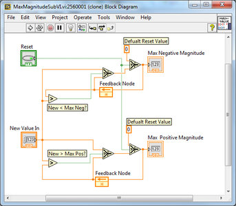
After the vectors are calculated the values are fed into MaxMagnitudeSubVI.vi. It spits out the largest positive and negative values its received. The code for this is depicted in the 2nd image. This vi consists of comparator, a couple of True False gates, and a Feedback Node. When a larger value I sensed by the comparator it triggers one of the TF gates to open. Once the new value passes through the gate it overwrites old value saved in the Feedback Node. A reset signal controls a gate that sets the Feedback Node to zero. Here is an example of what the MaxMagnitudeSubVI.vi looks like in action.

Step 3: 3D and 2D Vector Plot Code

All of the Vector plot code is implemented directly in the main PmodACL Plotting G-force Vectors.vi. This vi was built off of code from the previous projects.

The vector plots themselves are based on the vanilla ActiveX 3d Curve Graph.vi. This VI can be found by right clicking on the front panel then following the tabs, Classic->Graph->ActiveX 3d Curve Graph.vi. This VI accepts three 1-dimensional arrays. Each 1d array corresponds to one of the accelerometer's axes. For the plot to function properly these 1d array may only contain 3 elements. To get the vector to display correctly on the plot, the component vectors must be inserted into the center of the array (i.e array index 1). The arrays other two indices should contain zeros.

With the input arrays properly set up, next we need to configure the 3d plots to look how we want. All of the plots shown in the project are 3 dimensional plots. The plots which appear to be 2d are actually 3d plots, configured to display a single 2d plane. Aisde from differing perspectives, all the vector plots are configured the same way. I wont go into detail about how to configure each individual plot. Instead I will give an overview of how the plot configurations work. From there you can experiment and set up the plots how you like.

To start, here is how you open of the 3d plots configuration settings.

Here is show you make different grid planes visible.

Here is how you change the perspective of the plot.

Here is how you modify the plots axis labels and grid lines.

Here is how you get the vector line to appear on the plot.

Here is how you get the floating coordinates to follow the end of your vector line.

Here is how you get a 3D center-axis to appear on the plot.

That pretty much sums up how to configure the plots. You can try playing with the other settings to figure out the rest.