Introduction: 3D LED Cube
The 3D LED Cube is a really cool device that enables you to see in three dimensions, get some depth perception and has 512 LED's or 512 pixels. It is based on an arduino uno which is an Atmel AVR microcontroller on a development board with some standard interfacing pinouts that allow you to quickly assemble prototypes.
Step 1: 3D LED Cube Hardware
- The LED Matrix
- Control electronics for Columns
- Control electronics for Layers
By addressing the appropriate layer and column in the LED matrix, it is possible to switch a particular LED on or off or vary its intensity. For each of these sets of controls, we have an interface to the brain which is an arduino uno running an Atmel AVR microcontroller. The arduino uno is programmed via a USB port from a PC. The arduino uno brain (or AVR brain) contains standard interfacing pins which allow connection to the outside world and external devices.
Step 2: 3D LED Hardware - Control Electronics for Columns
Control electronics for Columns
To the interfacing pins on the arduino uno brain, we connect two PWM shields which are cascaded together in a long chain. Each of these PWM shields provides up to 32 pulse modulated outputs so these are the brightness controls for 64 columns in total (2 shields with 32 LED controls each). To light up a particular LED, we switch on that column and that layer at the same time to pinpoint an LED. Using this idea we can light up an entire column.
The PWM shield is designed to sync current so to turn on an LED, the PWM shield expects to be connected to the negative or cathode connection of the LED. However because of the way this cube has been wired, this chip has to interface with the positive or anode connection of each LED. In order to do this, you need to assemble an interposing transistor board. Using PMP transistors and sizing the current reference resistor on each PWM shield appropriately to compensate for transistor gain, we can provide a current source rahter than sync to each column. The column will source or supply the current via the positive anode to the LED and the common cathode layer will be sunk to ground using MOSFET.
Within each PWM shield, there are two TLC chips - arranged in a daisy chain serial communication fashion. There is a TLC chip library available from the arduino website which allows us to drive all this with minimal software coding. This library makes it easy for us to interface with this complex chip.
Step 3: 3D LED Hardware - Control Electronics for Layers
Control Electronics for Layers
To switch to layers we use a hardware d-multiplexer. We have three pins coming out of the arduino uno that are a binary coded decimal representation of the layer address. When you convert the binary coded decimal to a decimal you have 3 inputs into the d-multiplexer and 8 outputs on 0 - 7. Out of the hardware d-multiplexer we run a Darlington buffer which provides the current to quickly charge the gates of the MOSFET devices. Each power MOSFET (8 in total) conrols a layer and each layer has the potential of up to 1.6 amps of current so MOSFETS are the high power devices.
Step 4: 3D LED Software
Software for the LED cube is written in C and compiled under the arduino development environment. The code is transferred to the arduino uno via a USB cable so this requires a USB to serial converter to program the AVR directly.
The best way to think of the software is in two main parts:
- the philosophy of displaying the image
- the patterns and algorithms used to generate the image
The display philosophy allows us to only light up one layer of LED lights at a time, so in order to view the entire cube of LEDs simultaniously, we rely on a phenomenon known as Persistance of Vision. This is so we can scan through all of the LEDs or layers of LEDs without necessarily having them all on at one time. If we can scan through them fast enough, (typically 20 - 25 cycles per second or 8 layers 25 times per second) then they will appear to all be on at the same time.
In reality, because of the structure of the code, the cycle time will vary so the image or the current state of the image is represented by a 3 dimensional byte array. It is an array with the dimensions of 0 - 8 in all directions but realistically only 1 - 8 are used for the current state of display. The 0 address is used for manipulating row when we think about patterns and algorithms. Just focus on the 1 - 8 for each axis for now. This gives us 512 bytes of storage and each byte represents 0 - 255 grey scale value which then gets converted into a pulse with modulated representation of intensity.
On each loop of the program there is a nested loop which scans through the 3 dimensional array and writes one layer at a time. There is a preprogram delay which can be adjusted if need be which determines how long each layer is on for.
When you increase the speed of this scanning there are a couple of problems you can run into which is why we need to incorporate blanking on the d-multiplexer. By utilizing the d input for the d-multiplexer which exceeds the 3 - 8 specification, we can then blank all outputs of the d-multiplexer. This is what is connected to pin 7 of the arduino and is represented by the output value 128 because it is the most significant bit of a byte. As we scan the display faster, if we don't blank, we will a trailing of light through the layers where we don't actually want the light so the value of the previous layer will carry across onto the next one. We need to blank the layer control for a very short time while we write the new values to the columns, and then we can switch to the layer above and remove that ghosting affect.
One thing we have to be careful of when adjusting or compiling this code is the configuration of the TLC library. You need to look in the comments section of the source code provided to check what settings need to be changed in the TLC configuration file. When addressing the TLC chips the available library provides an interfacing functionwhich allows us to talk to the channel on the TLC system. In the library configuration file we specify that there are 4 TLC chips because there are 16 outputs per TLC chip. This allows us to drive 64 channels or 64 outputs simultaneously so these are addressed as channel 0 - 63. As we do our nested loop and scan through for a layer we need to consecutively write each value to each channel so there is a great deal of nesting or nested looping. Each LED is represented by 0 - 255 or 1 byte greyscale value. This is passed directly into the TLC function.
Step 5: 3D LED Software - Patterning
Patterns and algorithms are used to generate changes in the LED display. Upon each loop of the program we write consecutively 8 different layers. We can then perform mathematical manipulations on the array which contains image data. It can be done several ways:
- use an algorithm - like a nested loop which may generate some kind of repetitious pattern
- store a static image or a series of images or frames that will eventually make a movie by storing the states of the LEDs or brightnesses as a three dimensional array in flash because this is the non-volatile memory. We can store pixel by pixel data rather than having to generate it from an algorithm.
- Test Pattern - vary brightness of all LEDs using a sine function lookup table. You will get a nice smooth sinusoidal adjustment of the brightness. Therefore, we can determine if there are any faults or LEDs misbehaving in the first few seconds.Also it allows us to see if the program is functioning smoothly.
- Preset Pattern - initialized in 3 dimensional space using a bunch of formulas that sit in flash memory. This initializes with a bunch of objects and then there are a whole pile of transformation functionsincluded. On the first pattern these simply shift the image space or the mathematical image space down. When you do a transformation, you shift one row or one layer into the 0 address which is the temporary holding address. We can then shuffle all the values without losing any information. For example, we can take information off the top, shift the whole display up and take the information from the top and place it on the bottom. We can have a repeating pattern that feeds back into itself si it appears as if it is continuously moving up (or down or left or right).
- Randomized Transformation - we use that same space in the next pattern and shift to a randomized transformation. We randomly assign a transformation or a combination of transformations which gives the appearence of a space randomly moving or vibrating about.
- Randomized Rain Pattern - shows a downward transformation recurring but as this is happening, we randomly make changes to the space so it doesn't seem to be looping over itself and its constantly evolving.
- Greyscale Representation of a Sinusoid - we use the sine function lookup table to determine the brightness of each particular LED based on a constantly changing angle. This angle is fed into the sine function and on each iteration of the loop, the angle is increased till you get a constantly varying sine function using intensity.
- Sine Function - instead of using brightness, it notes the nearest LED to that value. Think of a sine wave superimposed onto the side of the cube and round to the nearest LED but as this moves quite fast, it gives the appearance of a nice sine wave. We also incorporated a bivariate function which is constantly morphing as the program loops through and allows us to change the direction of this particular sine wave.
- Motion of a Particle or Ball - it is like a simple physica engine which simulates the motion of a particle or ball exposed to acceleration due to gravity and drag - it eventually slows. It is also exposed to interference rules on all sides of the cube apart from the roof so this allows the particle to shoot out of the space and re-enter, confined by the walls and the floor. This has a trailing decaying tail behind it which allows you to see the trajectory a lot better.


