Using the Oscilloscope With the Analog Discovery 2

Oscilloscopes are used to graphically display time varying signals, with time as the independent variable on the x-axis, and the dependent variable, such as voltage or current, on the y-axis. They are incredibly useful, but bench top scopes can be large and bulky, and break the bank at the same time. The Analog Discover 2 aims to alleviate both problems, being at once affordable as well as compact and lightweight.

For this Instructable you will need:

- 1X 100μF electrolytic capacitor

- 1X 20kΩ

- 1X 9V battery w/ battery clip

- 1X breadboard w/ jumper wires

-Analog Discovery 2*

-Waveforms 2015 software*

- a computer with USB port to run the software

*You may also use the original Analog Discovery or the Electronics Explorer Board with Waveforms 2015. There are some slight differences in functionality between the AD1, AD2, and EEBoard, but nothing that will prevent you from following along if you have one of the other tools.

Step 1: The Oscilloscope

There isn't much background to oscilloscopes, so let's just dive right in. If you want some help with AD2 calibration and Waveforms installation/setup, check out this quick start I'ble collection.

Before we get to using the AD2, we need a simple time-dependent circuit so we can see what's going on.

When the switch is closed, the capacitor charges but quickly reaches full capacity. Once it does, it acts like an open break in the wire and the voltage across the resistor is the same voltage as the battery. Once the switch opens, the capacitor starts to drain through the resistor. The equation Τ = RC tells us that it will take Τ (Greek Tau) seconds for the capacitor to drain to ~36.8% of it's previous value. For our schematic, we get Τ = 20kΩ * 100μF = 2s. We'll come back to this value in a bit.

Connect the 30-pin connector to the AD2. Connect "1+" to the capacitor anode (+) and connect "1-" to the capacitor cathode (-). Because the oscilloscope channels on the AD2 are fully differential, meaning that they can measure differences in potential between the "1+" and "1-" pins with no need for a GND reference, there is no need to connect a GND wire from the AD2, though you may if you wish. If you use the Electronics Explorer Board, the scope channels are not differential so you will need to connect one channel to the anode and GND to the cathode. In this example that also connects to the "-" battery terminal.

Your circuit should look something like this once you have it all set up.

Once you have your AD2 and circuit set up, open Waveforms and click on the "Scope" button at the top.

The Oscilloscope window will open.

Step 2: Capturing Data.

Make sure your switch is turned off, then go to the scope window and click to start acquiring data. You should see a blue line at 0 and nothing else.

Turn off the switch, and you'll see the yellow line start to fall into view, eventually settling back down at 0.

Clearly we need to make some adjustments to the viewing window. If you look at the y-axis, you'll see that it only goes up to 2.5V, with each division set at 500mV/division. Since we are using a 9V battery, we're going to miss data when the capacitor is charged to 9V.

Go to the right side of the window where you see options for adjusting channel 1 and channel 2.

Clicking on will allow you to turn off the trace on the plot for whichever channel you select. Since we don't have channel 2 in use here, we can deselect it here.

In the channel 1 box, we have a couple of different options. We can give our trace an offset, which will move 0 in that direction. If you enter a value of "-5V" here, it will move 0 on the plot down 5 volts. You end up with +5V at the center of the plot on the y-axis. If it's confusing, don't feel bad. It took me some time to figure out what value to enter for which direction as well.

The range box lets you set the scale for the y-axis. Since we are using a 9V battery, let's set our range to "1V/div". You can click on the drop down arrow, or enter it directly into the box.

The plot window is hard coded to divide both the x- and y-axis into 10 divisions. With a -5V offset (centered on +5V) and 1V/div scale, we get the y-axis displaying 0-10V. Click again and switch on your battery. You'll see the channel 1 trace jump to about +9V. Switch off the circuit and you'll see the trace slowly start to fall. We're getting closer to capturing all of the data. But let's see if we can't capture all of the data by adjusting the x-axis.

Take a look at the time adjustment box. You can adjust the position, and unlike the channel offset, the value you enter here will be the value that is placed in the center of the x-axis. You can also set the time per division. Let's leave the position at 0 and set the the base to 2 s/div.

Make sure your switch is off for at least 20 s, then click to start acquiring data. A vertical gray bar will slowly move across the plot window and the channel 1 trace will start to plot along the bottom at 0V. Wait a few seconds then close the switch. You will see the trace jump very quickly up to about 9V, showing that the capacitor charges very quickly.

You'll also notice that once the trace reaches the far right side of the window, it will wrap around to the left and start overwriting the trace data that is there with the current data. If you need to acquire more data for a longer time, you can adjust the time window. You can adjust it back down later to zoom, but remember that the plot can only take a set number of data points for the entire width of the plot window. If you zoom in after stopping the acquisition, the space between data points spreads out and the resolution of your data is degraded. I'll go over some tips on how to zoom while still viewing the data in a bit. This particular circuit is a bit too slow to show that.

Let's capture a specific window of data. Make sure that the switch is on. Click again, but this time turn off the switch after about 2 seconds. Let the gray bar move all the way to the right and then click before it wraps around to the left side of the plot. You should get something like this.

Step 3: Interpreting the Data.

OK, there are a lot of things we can do with the data we captured. Remember our value for the time constant Τ? Τ = R * C = 20kΩ * 100μF = 2s. Let's see how that worked out. First we need to determine our max value. By visual inspection, I guess the value to be about 8.78V. The problem is that it's just that, a guess.

Go to the top and click on "View". There are a ton of options here, but click on "Measure". We also need to open the "X Cursors" pane, so open that from the same menu.

The Measurements pane will open up to the right of the plot window, while the X Cursors pane will open below the plot.

In the top right corner of these panes you have some small buttons. Clicking will close the window, so don't do that yet. If you do accidentally close a pane, the changes you made will be saved as long as you don't close the program. Just reopen the pane. Clicking will allow you to pop out the pane into its own window. The panes make the plot area smaller, so this may make viewing the plotted data easier. You can also click and drag on between each pane and the plot to adjust the pane size without popping it out to a window. If you want to place the window back into the scope window, you can click on the top of the window, and dragging it around the scope window will highlight different areas where you can place the pane. Your choice.

In the Measurements pane, click and then "Defined Measurement" to add a measurement option. Make sure Channel 1 is selected, then double click on "Vertical" and then either double click "Maximum" or click it once then click "Add". The "Add" window will stay open either way, so close it once you're done adding measurements.

If you end up adding too many of the same measurement, or are done with one, make sure that particular measurement is highlighted by clicking on it, then click on at the top of the window. A small window will open.

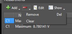
"Remove" will remove just that one channel. "Clear" will remove all measurement channels. The "Edit" button will allow you to edit the background software code that is assigned to that specific channel. There is no need to do that for this example, but this is handy for making custom measurement channels that involve some sort of math function, like determining current through a resistor by measuring just the voltage. The "Show" button will add different metrics to each measurement channel. These could be useful for determining consistency in a signal. We are only concerned with the value here, so we'll leave that alone as well.

Now to the "X Cursors" pane. Click to add a vertical cursor on the x-axis on the plot. Clicking either again or will add more cursors. Let's add 2 cursors. These cursors can show data that is dependent on the data from another cursor, or just the raw data at that point. You can click on at the bottom of the cursor line to move it around. The data will display both in the X Cursor window as well as on little labels on the plot. If you click on the small arrow to the right of the number on the cursor, a small option window will open. These options are the same as what you see in the X Cursor pane, allowing you to set them in both places. You can also change the cursor color here.

For this example, we want cursor 2 to show the change in voltage for a set time between it and cursor 1. Make sure that the "Ref" column says "none" for cursor 1 and "1" for cursor 2. Also enter a value of 2s in the column marked "ΔX" for cursor 2. "Δ" means "change in", and this is the change in X we want between our two cursors. This will set cursor 2 +2s ahead of cursor 1 (entering "-2" will put cursor 2 -2s behind cursor 1). If you click on cursor 1 and move it around, cursor 2 will move with it, always maintaining ΔX at 2s since cursor 2 is dependent on cursor 1. Moving cursor 2 in the same way will not move cursor 1, but will change the value of ΔX.

Move cursor 1 to a point on the plot where the value for C1 has to dropped below the value shown for C1 Max in our measurement. For my plot, that is anywhere to the right of -8s.

Look at the values for cursors 1 and 2 in the cursor window. I have 8.5560V for cursor 1 and 3.2284V for cursor 2 when cursor 2 is 2s after cursor 1. Remember our value of Τ = 2s and what it meant? It's the time it takes for the charge across the capacitor to drop to ~36.8% of its previous value, and this % will hold for any 2 second window we measure. 3.2284V / 8.5560V = 0.3773 = 37.73%. This error is easily accounted for when we consider that we assumed nominal values for our components (20kΩ and 100μF) were actual values, so we are right where we should be. Now, go to the Position column for cursor 1 and type in any other value that is in the plot, e.g. -3.702s. Since we locked ΔX for cursor 2 at +2s after cursor 1, the cursors will move on their own and my plot shows values of 1.0716V for cursor 1 and 0.4139V for cursor 2. This gives a drop to (0.4139V / 1.0716V) = 0.3875 = 38.75% of 1.0716V, which is within expected error.

Now let's take a look at some of the other functions we have access to with the oscilloscope window.

Step 4: Some Additional Functions.

Pressing "F1" on your keyboard will open up the Help menu for whatever tool you have open. You can also click "Window" at the very top left, then on "Help". In several locations throughout Waveforms 2015 you'll see . This is a generic icon used to denote where you can make changes to various settings. There are too many options to go through every one of them here, but a couple in particular are very useful in general so let's look at them now.

One is triggering, which is often used to force the scope to only capture data if a certain type if input condition is met. At the top of the window there is a small green arrow . Clicking on it will open some more options on the top tool bar, most of which apply to the triggering capability.

The "Mode" box lets you change how the data is displayed, either one full plot at a time, real-time that wraps around once the end is reached, real-time side-scrolling, or record. The "Screen" setting here is fine. The box that says "Auto" next to the word "Source" lets us determine how we want the trigger to acquire data. "Auto" will acquire enough data to fill the plot window one time for whatever data present if the trigger condition has not been met for 2 seconds. "Normal" will only acquire data if the specified trigger condition is met. "None" will ignore trigger settings and just acquire data.

From the "Source" box you can select various trigger sources, including other AD2 tools like one of the Wavegen channels, or even an external source. The "Type" box will let you choose what type of signal change (edge, pulse, or transition) you are wanting to use to trigger the scope. Choosing either pulse or transition will change the options available in the Condition and LCondition boxes. The "Condition" box lets you further define what type of signal you are looking for. For example, you choose "Edge" for type, but are you expecting a rising or falling edge? Or you choose "Pulse" for type, but do you want a positive or negative pulse? "LCondition" will let you further define "Pulse" and "Transition" triggers.

In the "Level" box you can set the vertical level where you want the trigger to happen. If you are looking for a spike of data, set the level above the noise to ignore everything but the large spike. "Length" specifies the minimum or maximum pulse length or transition time for either "Pulse" or "Transition" types. The "Hysteresis" box is extremely useful for signals that have a lot of small oscillations that are contained within much larger oscillations, like when you add two sine waves whose frequencies are at least an order of magnitude or more apart. The "Auto" option here should be fine for nearly every type of signal. "Holdoff" allows you to tell the trigger to wait for a specific amount of time so that the data can acquire properly.

For this example, I've set my trigger with the following settings:

I've also changed the Time base setting to 10ms/div. The goal is to capture the data from the capacitor charging. Make sure your switch is off for at least 20 seconds, then click "Run". The "Run" button should be a "Stop" button and right below it you should see . This tells you that the trigger is armed and waiting for the specified condition. Close the switch and you should acquire one full plot of data, showing the voltage across the capacitor as it charges.

Here we can clearly see the switch bounce that is very common in mechanical switches.

You can adjust the scales for the x- and y-axes while using the trigger. The first instance that the trigger conditions are met will be centered at the point where the trigger level and 0s intersect. On the plot you can see these marked by the yellow triangle on the right set at 3V and the white triangle at the top at 0s. You can click and drag on either of these to move the plot around. Entering a value in the "Position" box in the Time settings window will move 0s, even off the plot if you wish. The first instance that the trigger conditions are met will STILL be centered at the point where the trigger level and 0s intersect, even if you put 0s off of the plot.

Here I've set the time position to 6 ms, which moved the trigger instance out of view to the left.

As long as you don't press the "Stop" button at the top, the scope will go back to the armed trigger condition and wait for another instance that satisfies the trigger specifications, at which point another round of data will be acquired and displayed.

Another very useful function is being able to add a math channel to the plot. This allows us to manipulate the data with math functions to see it in a different way. For this, let's reset to our previous settings. Examine the image carefully, set your scope window to match, and capture one plot worth of data of the capacitor discharging like we did before. Be sure to set the "Mode" box at the top to "Screen" and the trigger to "None".

Between the Time and Channel 1 boxes on the far right you'll see . Click on it, then choose "Custom". A new trace will appear on the plot and a new math channel, M1, will appear below Channel 2.

Click on the math function button to open the math function editor.

Let's use this to determine how much current is passing through the 20kΩ resistor. Since current is found by dividing voltage by resistance, I = V / R, we need to divide our voltage (C1) by the value of the resistor (20000). Replace "pow(C1,3)" with "C1 / 20000". In the units box, enter either "Amps" or "A" since we are trying to measure current, then click "OK". Now let's adjust our window settings so we can see our trace. A quick way to do this is to divide the settings for Channel 1 by 20,000, so we get -0.00025 A for our offset 0.00005 A/div for the range. Since the default is several orders of magnitude larger than these values, the program has a hard time letting you enter very small values for the offset unless the range is in the same order of magnitude. Enter the value for the range as "0.00005A" and press enter. This will allow you to type in "-250uA" for the offset. You should see the Math trace overlap the trace for Channel 1. To see them both clearly, you can adjust the offset for M1 to "-200uA", or you can click on the y-axis numbers and drag the scale to where you want it. If you want to move the C1 scale, click on C1 at the top left of the plot to select the C1 scale, then click and drag on the axis as needed. You should end up with something like this:

Since resistors are linear devices, we see that the current through the resistor exactly tracks with the voltage applied to it.

How much power is our resistor dissipating? I've used a 1/8th W (125mW) resistor, so should I be concerned that I'm reaching it's max limit? I seriously doubt it, but let's add another math channel to find out. Don't delete M1, just add M2. By manipulating Ohm's Law, there are three functions we can use with the data we now have, W = V * I, W = I² * R, or W = V² / R. In the function editor window, enter the function that works best for you, remembering that we found the current I with channel M1. I entered "sqr(M1) * 20000", which is I² x R. In the units box enter "W" and click "OK". You'll need to adjust your scale for M2 as well. I found that an offset of "-2.5mW" and a range of "500uW/div" worked well. You can use either a cursor or the measurement pane to determine the max value. You should see the following:

You can see that along the cursor, M2 shows a value of 3.854mW, which is well below our max allowed value of 125mW, so we are more than OK here. You can also see that the power dissipated is not linear at all, which should be apparent from the exponents in the equations derived from Ohm's Law.

Step 5: Using the BNC Adapter.

By attaching the BNC Adapter Board to your AD2, you can use standard BNC-terminated probes and test leads.

There are some things to keep in mind when using the BNC board and BNC probes. Most probes can attenuate the signal, usually by a factor of 10X or even 100X.

This is useful when your input signal is higher than your scope can display. The AD2 oscilloscope too can only display a maximum of 50V peak-to-peak, so if your signal was 400V, which my leads can handle but the scope can't display, I can set the switch to 10X and I will read 40V on the scope image. That being said, it's easy to forget that you set your probe to 10X and then you go to read some data and it is way smaller than expected.

Here we see the same exact signal with two different probes. Channel 1 is set to 1X and Channel 2 is set to 10X, so it displays a signal that is 1/10th of actual.

You can switch the probe to 1X, or you can adjust the attenuation in the channel settings.

With the settings box, you could feasibly attenuate a signal over 1000X if your probe is set at 100X and you set the scope channel to 0.1X attenuation in the settings box.

The BNC adapter board has a small jumper behind the BNC connector that will allow you to choose between AC or DC coupling. If your circuit is a DC circuit, you want it DC coupled. However, if your signal has some kind of AC sinusoidal signal, it may be beneficial to switch to AC coupled. This will remove any DC offset and center the sinusoidal signal at 0 magnitude. For our purposes, we will leave it DC coupled.

Also be sure to connect your probe to circuit GND. Weird stuff can happen if you don't, so if you get weird stuff, check to make sure your probe GND is properly connected.

Step 6: I Think That's Good for Now.

I've covered a lot of information on how to use the oscilloscope, and these are really the basics for using any oscilloscope. It can be confusing and hard to remember, but with the combination of Waveforms 2015 and the Analog Discovery 2, and a little bit of practice, data acquisition is much simpler and can be done at a much lower cost than with traditional bench top tools.

As always, thanks for reading. If you have questions, please ask them in the comments below, though PM's are always welcome as well. You just never know when someone else has the same question and that way we can all learn and help each other get better. Have fun building!

Also, please check out the Digilent blog where I contribute from time to time.